WAN Optimization: TCP Congestion Control Algorithm Technology White Paper

 

 

 

 

 

 

 

 

 

 

 

 

 

 

 

 

 

 

 

 

 

 

 

 

 

 

 

 

 

 

 

 

Contents

Overview·· 1

Technical background· 1

Application of congestion control algorithms in WANs· 2

Operating mechanism of the congestion control algorithm in WAN· 2

Congestion control algorithm metrics· 3

Basics of TCP·· 3

Concepts· 3

TCP acknowlegement mechanism·· 4

Sliding window· 5

Introduction to the sliding window mechanism·· 5

Transmit window, receive window, and congestion window· 6

TCP retransmission mechanism·· 7

Reno and BIC algorithms· 8

Principles of Reno and BIC algorithms· 8

Slow start phase· 8

Fast retransmission phase· 9

Rapid restoration phase· 9

Congestion avoidance phase· 9

Differences between Reno and BIC algorithms· 9

Summary of Reno and BIC algorithms· 11

BBR·· 11

Concepts· 11

Principle of BBR algorithm·· 12

Implementation process of BBR· 13

StartUP (Startup phase) 13

Drain state· 13

ProbeBW state (during the BtlBw sniffer section) 14

ProbeRTT state (RTprop sniffer section) 14

BBR algorithm summary· 14

Introduction to BBRv2· 15

Comparison of congestion control algorithms· 16

 

Overview

Technical background

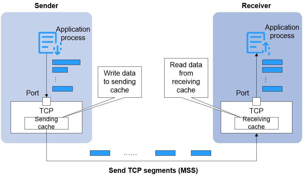
TCP is a transport layer protocol in the TCP/IP system, providing connection-oriented and reliable services for applications. TCP ensures the reliability of message transmission by using sequence numbers, acknowlegements, and timeout retransmissions. As shown in Figure 1, the TCP data transfer process is roughly as follows:

1.     The application process at the transmitting end continually generates data (the size of the data blocks might vary) and writes these data blocks into the TCP's transmit (Tx) buffer.

2.     TCP regards the data blocks to be transmitted as a data flow composed of byte groups, and allocates a sequence number for each byte. The TCP protocol stack extracts a certain amount of data from the transmit cache, composing it into a MSS (Maximum Segment Size) to be sent out.

3.     After the receiver receives the TCP segment, it temporarily stores it in the receive buffer.

4.     The application process at the receiver end reads data blocks one by one from the receive buffer.

Figure 1 TCP transmiting MSS

 

If the transmitting end sends data too slowly, it can waste network bandwidth, affect process-to-process communication, and even cause communication failure. Therefore, we aim to deliver the data to the receiving end as quickly as possible. However, if the transmission is too fast, the receiving end may not keep up, resulting in data loss. The congestion control algorithm controls the number of TCP packets that the sending end can transmit through a complex mechanism. This ensures the transmission rate is not too fast for the receiving end to handle and not too slow to waste bandwidth and affect business. Thus, it maximizes the use of network bandwidth, improves transmission efficiency, and minimizes data loss. It also ensures TCP packets are delivered to the receiving end promptly, reducing transmission delay.

Application of congestion control algorithms in WANs

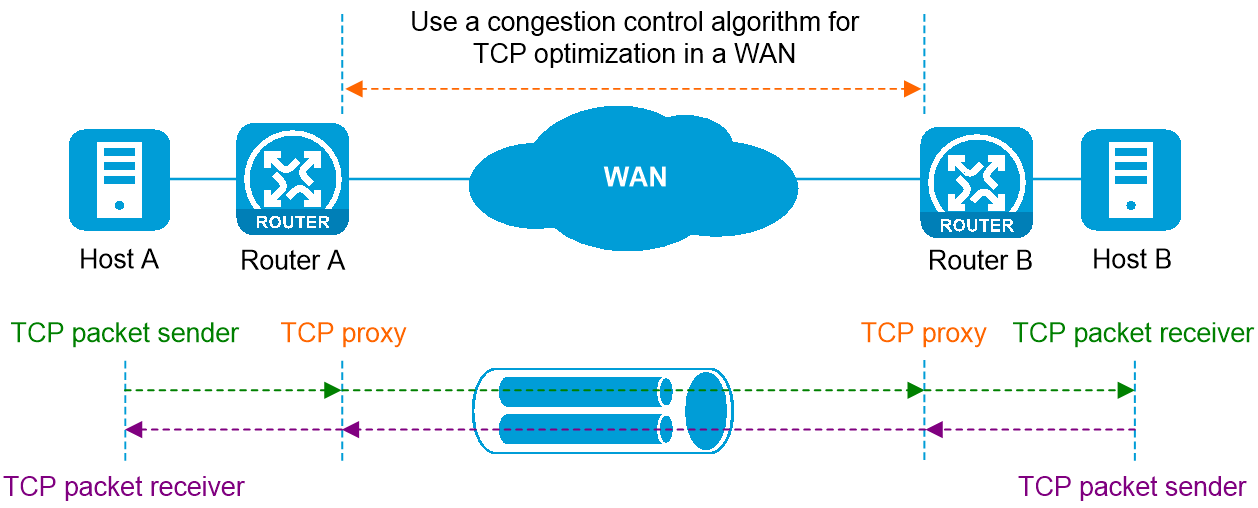
As shown in Figure 2, when Host A accesses Host B via the Telnet protocol, a TCP connection is established between Host A and Host B, and Router A and Router B forward the TCP packets. Normally, local area network (LAN) bandwidth is sufficient, and TCP communication performance can be ensured even without running a congestion control algorithm. However, for wide area networks (WAN), issues such as complex network structure, long physical transmission distances, and lower transmission rates compared to LANs result in high WAN latency, low bandwidth utilization, and high packet loss rates, significantly reducing the performance of TCP communication in WANs. To solve this problem, we deploy a congestion control algorithm on the WAN access devices (Router A and Router B), which can achieve the following: regardless of whether the sending end of the TCP session supports the congestion control algorithm, Router A and Router B can ensure that the original TCP packets make optimal use of WAN bandwidth without causing network congestion and quickly reach the receiving end while traversing the WAN.

This article mainly discusses the application of congestion control algorithms in wide area networks (WAN).

Figure 2 Implement the congestion control algorithm for wide area network (WAN) TCP optimization

 

Operating mechanism of the congestion control algorithm in WAN

As shown in Figure 2, the wide area network (WAN) congestion control algorithm is deployed on access devices Router A and Router B, and is used to control the number of TCP packets that Router A and Router B can transmit. The operating mechanism is as follows:

1.     The administrator configures the wide area network (WAN) optimization policy and deploys the congestion control algorithm on Router A and Router B. After this, Router A and Router B each automatically create a TCP Proxy.

2.     Host A initiates a TCP connection request (CR) to Host B, establishing a TCP connection.

3.     The TCP Proxy on Router A and Router B matches the TCP connection establishment request between Host A and Host B based on configured rules, and creates a proxy TCP connection between Router A and Router B.

4.     Router A receives the original TCP message sent from Host A to Host B. The TCP Proxy on Router A encapsulates this original TCP message as a data block into a new TCP message, which is then transmitted over the proxy TCP connection. The congestion control algorithm on Router A controls the number of TCP messages that can be transmitted from the local end on the proxy TCP connection.

5.     Router B receives the original TCP message from Host B to Host A. The TCP Proxy on Router B encapsulates this original TCP message into a new TCP message as a data block for transmission on the proxy TCP connection. The congestion control algorithm on Router B regulates the number of TCP messages that can be sent on the local end of the proxy TCP connection.

The number of messages that can be transmitted each time by the sender is determined by the congestion control algorithm. Reno, BIC, BBR are the three mainstream TCP congestion control algorithms supported by Comware. Different algorithms have different principles and scenarios of use.

 

NOTE: This article only theoretically explains the basic principles, mechanisms, advantages, and disadvantages of the Reno, BIC, and BBR algorithms to help users select the appropriate congestion control algorithm. In practice, different manufacturers adjust the parameters of these algorithms, so please refer to the actual situation.

 

Congestion control algorithm metrics

The computer network environment is intricate and constantly changing. The TCP congestion control algorithm is continuously evolving to seek for better solutions for bandwidth, package loss, and delay. Two important metrics measure the effectiveness of the congestion control algorithm.

·     Bandwidth Utilization: This refers to whether the algorithm can quickly find the maximum number of packets that can be transmitted each time when the network is idle, to maximize the use of network bandwidth, increase the transmission rate, and improve communication efficiency.

·     Fairness: This refers to whether the algorithm can fairly allocate bandwidth among various TCP connections. For example, when a new session joins competing for network bandwidth, the algorithm should enable existing TCP connections to yield some bandwidth, so that new connections can fairly share bandwidth with old ones.

An algorithm that has a high bandwidth utilization and good fairness is more superior.

Basics of TCP

The congestion control algorithm is based on TCP validation responses, sliding window mechanisms, and so on. Sequence numbers and MSS are frequently mentioned in the congestion control algorithm. To facilitate understanding of the technical implementation of Reno, BIC, and BBR congestion control algorithms, let's first review the TCP fundamentals that are closely related to the congestion control algorithm.

Concepts

Sequence number

The sequence number is a field in the TCP message header, used to indicate the sequence number of the first byte of data transmitted in this message section.

TCP is oriented towards data flow, and the packets transmitted by TCP can be seen as a consecutive data flow. TCP assigns a sequence number to each byte in the data flow transmitted in a TCP connection. The initial sequence number of the whole data flow is set during the connection establishment of TCP.

TCP segment

TCP transfers the data flow generated by the application layer in segments. These segments are encapsulated in the data part of the TCP package. A section can contain multiple bytes of application layer data.

MSS

MSS indicates that the maximum length of the message segment a device can receive is MSS bytes. During TCP connection establishment, the transmission end and the reception end write their respective MSS values into the option field of the TCP header generated by their end to inform the other end of their processing capability. Both parties select the smaller MSS as the MSS value for this TCP communication.

For ease of description, this document also uses MSS in place of the term 'section of a message'.

RTT

The time required for a TCP packet to travel from the sender to the receiver and back is known as RTT (Round-Trip Time). This is calculated through the interaction of TCP packets.

Retransmission tmeout

The transmission end begins by transmitting a packet section, up until the interval time before this section is retransmitted. Typically, the transmission end sets the RTO as a value slightly larger than the RTT.

Transmit window

The transmit window is a buffer block established within the operating system by the sender to store the current data to be transmitted, also known as the transmission buffer. The sender uses the transmit window for traffic control.

Receiver window

The receive window is a buffer block opened within the operating system by the receiver, where the device places incoming packets that haven't been processed yet, also known as a receive buffer. The receiver uses the receive window for traffic control.

Congestion window

The congestion window is a value set by the transmitting end based on its estimation of network congestion. The transmitting end uses the congestion window for traffic control.

TCP acknowlegement mechanism

TCP is a connection-oriented, reliable stream protocol. It improves reliability by using sequence numbers and acknowlegements. The TCP acknowlegement mechanism is as follows:

1.     The sender divides the business stream into data blocks that are most suitable for the current network transmission, adds a sequence number to each byte, and then transmits them in MSS units. A transmission timer is also started.

2.     After the receiving end receives the MSS message section, it replies with an ACK message carrying a validation sequence number (validation sequence number = the largest sequence number N+1 in the continuously received messages). The validation sequence number indicates that the message with sequence number N and the ones before have all been received. Please transmit a message with the sequence number N+1.

3.     Once the transmitting end receives the ACK, it can transmit the next MSS. The waiting time involved is one Round-Trip Time (RTT). If the ACK message is not received when the transmission timer times out, the MSS will be retransmitted.

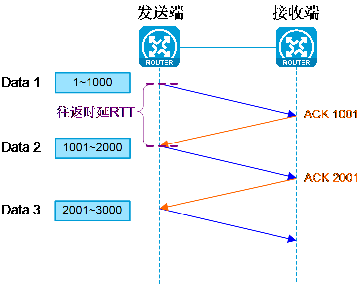
As shown in Figure 3, assuming the MSS is 1000 bytes, the transmitter sends one MSS of data each time and can only send the next MSS after receiving the acknowledgement (ACK) response from the receiver. In this way, the transmitter sends one MSS after one round-trip time (RTT). When the RTT value is larger, the network throughput will be worse, and the transmitter spends most of its time waiting for ACKs. To solve this problem, TCP introduces the sliding window mechanism.

Figure 3 TCP validation answering machine mechanism

 

Sliding window

Introduction to the sliding window mechanism

To address the issue of low transmission rate caused by the validation answering machine in TCP, the sliding window mechanism was introduced into TCP.

The sliding window is a section of memory used to store message segments. The size of the window refers to the number of message segments (MSS) that can be transmitted continuously without waiting for validation responses.

The core concept of the sliding window is that TCP enhances its transmission rate by parallel transmitting data sections within the sliding window.

The specific method to implement a sliding window is:

1.     The application layer at the transmitting end stores the generated data in the sliding window.

2.     When the transmitter sends data, it no longer transmits one message section (MSS) at a time. Instead, it can transmit any message section within the transmit window range without waiting for the ACK of the previous data package.

3.     Each time TCP receives a validation response for a message section, it removes the message section from the transmission window and slides the window forward by the length of one section. This readies the sender for the transmission of the next section. Any sent sections that have not yet received a validation response must be reserved in the window for potential retransmission.

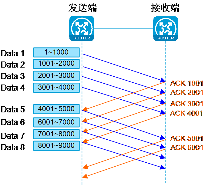
As shown in <field name="Ref" value="Figure 4"/>, it is assumed that the size of the sliding window is 4 MSS, with each MSS being 1000 bytes. Without receiving a validation response, the transmitting end can send Data 1, 2, 3, and 4. Once ACK 1001 is received, the sliding window can advance one MSS and Data 5 can be transmitted.

Figure 4 Use the validation retransmission mechanism after using the sliding window

 

Transmit window, receive window, and congestion window

In the sliding window mechanism, three important concepts are involved:

·     Transmit Window

The transmit window is a buffer block allocated by the sending end within the operating system for storing the current data to be transmitted, also known as the transmit cache. The sending end uses the transmit window for traffic control.

·     Receiver Window

The receive window is a buffer block opened within the operating system at the receiving end. The device places received messages, which it doesn't have time to process, into this receive buffer, also known as the receive cache. The receiving end uses the receive window for traffic control.

·     Congestion Window (CWIND).

The congestion window is a window value set by the transmitting side based on its estimation of network congestion. The transmitter uses the congestion window for traffic control.

In typical TCP communication, which is bidirectional, each device simultaneously has a transmit (Tx) window and a receive (Rx) window.

How is the size of the sliding window determined?

·     The size of the receive window equals the size of the current receive buffer at the receiving end, indicating the ability of the receiving end to receive packets at present. The receiving end places this window value in the window (WIN) field of the TCP packet header and transmits it to the sending end.

·     The principle for determining the congestion window is: if the network is not congested, the transmitter increases the congestion window slightly to facilitate more data transmission; if the network is congested, the transmitter decreases the congestion window slightly to reduce data transmission. How to judge whether the network is congested, and the degree of increase or decrease of the congestion window are all determined by the congestion control algorithm. The details will be described below.

·     In most cases, the transmission and reception ends are linked via network transmission equipment such as switches and routers, each with differing capabilities for reception and processing. Additionally, the link rates between these devices can also vary. As such, the transmit window size is determined by both the receiving capability of the receiving end (that is, the size of the receive window) and the transmission capability of the network (that is, the congestion window size).

The size of the transmit window is equal to the minimum value between the receive window and the congestion window. In other words, the size of the transmit window is determined by whichever is smaller – the receive window or the congestion window.

¡     When the receive (Rx) window is smaller than the congestion window, the receiving end's ability to receive limits the size of the transmit (Tx) window.

¡     When the congestion window is smaller than the receive window, the network congestion limits the size of the transmit window.

 

NOTE: For the TCP connection established between wide area network (WAN) devices, both the transmitter and the receiver are WAN devices, and the receive buffer of a WAN device is large enough (ranging from several tens to tens of thousands of KB, which users can configure through the command line). It is therefore much larger than the size of the congestion window. Consequently, the transmit (Tx) window of the WAN device is only constrained by the congestion window, taking the size of the congestion window directly.

 

TCP retransmission mechanism

TCP uses two types of message retransmission mechanisms: timeout retransmission and fast retransmission.

Timeout retransmission

When the transmitting end sends out a message segment, it sets up a retransmission timer and starts timing. The first set Retransmission TimeOut (RTO) is slightly larger than the Round-Trip Time (RTT) of the message from the transmitting end to the receiving end. If the segment's validation response (ACK) has not been received when the retransmission timer times out, the transmitter assumes the segment has been lost and retransmits it. If this retransmitted message also times out, the transmitter considers the network condition to have deteriorated, resulting in a doubled retransmission timeout.

The timeout retransmission mechanism of the TCP protocol can provide reliable transmission for applications. However, if the network is congested, especially in a wide area network (WAN) with high packet loss rate and transmission delay, validation waiting and message retransmission can greatly reduce network throughput and transmission efficiency, exacerbate network congestion, and even cause transmission disruption.

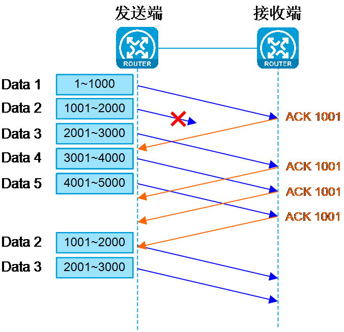
Fast retransmission

The Fast Retransmit mechanism operates not based on time, but on data to drive retransmission.

When the transmitter sends out the message segment, it sets up a retransmission timer and starts timing. The initial timeout retransmission time is slightly longer than the round-trip time (RTT) from the transmitter to the receiver. If the receiver does not receive the expected message segment within the specified time, it will continuously send three ACK messages with the same sequence number to the transmitter. Upon receiving three identical ACK messages, the transmitter will retransmit the lost message segment before the retransmission timer times out, greatly enhancing the efficiency of the retransmission.

As shown in Figure 5, assume the MSS is 1000 bytes, and the sliding window at the transmitting end is 4 MSS. If Data 2 is lost, the receiving end will respond with ACK 1001, requesting retransmission of Data 2. After the transmitting end receives ACK 1001 three times in a row, it initiates the fast retransmission mechanism to resend Data 2 to 5.

Figure 5 The mechanism of TCP fast retransmission

 

Reno and BIC algorithms

Principles of Reno and BIC algorithms

The Reno and BIC algorithms leverage package loss feedback, permitting the transmit end to passively adjust the size of the congestion window to control the quantity of the network package sections (MSS) that can be sent. This approach enhances bandwidth utilization and prevents network congestion. Both these algorithms incorporate four stages: slow start, fast retransmission, quick restoration, and congestion avoidance.

Slow start phase

After the TCP connection establishment, the algorithm kicks off and enters the slow start phase. The principle of slow start is as follows: When the transmit (Tx) end starts sending data, if all the section in the large transmit window is directly transmitted into the network without understanding the network status, it could lead to network congestion. Thus, slow start uses a sniffer method, gradually increasing the congestion window value from small to large at the transmit end, to determine the ideal congestion window size for current network transmission.

The specific approach to slow start is:

·     The TCP process begins sending packets at a lower rate (with the corresponding congestion window CWND being one MSS), and then doubles the CWND after each round-trip delay RTT, in order to quickly sniff out the optimal CWND.

·     At the same time, the algorithm sets the slow start threshold (ssthresh) with an initial value of 256 MSS. Ssthresh is used to prevent the congestion window from growing too fast without restrictions, which can cause network congestion. If CWND is greater than or equal to ssthresh and the network is still not dropping packages, it will directly enter the congestion avoidance stage and start to grow the congestion window slowly.

Fast retransmission phase

The continuous increase in the congestion window CWND inevitably leads to network congestion resulting in package loss. If the transmitting end continuously receives three ACK messages with the same sequence number, the TCP process will assume the current network congestion causes package loss. The algorithm then enters the fast retransmission stage and immediately retransmits the message section not yet received by the recipient, without waiting for the ACK message to timeout before retransmission.

Rapid restoration phase

Fast recovery is usually used in conjunction with fast retransmission. After the fast retransmission, the algorithm enters the fast recovery phase. Without using the fast recovery mechanism, the sender, when detecting network congestion, reduces the congestion window to 1 MSS and starts the slow start phase. This approach is quite extreme, as in reality the network isn't congested to the extent of only being able to transmit one MSS. This leads to the TCP transmission rate not being able to quickly return to normal state. To solve this problem, TCP developed the fast recovery mechanism. During the fast recovery phase:

·     The algorithm reduces the congestion window CWND to half of the CWND when packet loss occurs, to quickly alleviate network congestion and restore smooth network flow.

·     Simultaneously, the algorithm sets the slow start threshold (ssthresh) as half of the congestion window when the package is lost, to enter the congestion avoidance stage.

Congestion avoidance phase

During the congestion avoidance phase, the slow-start threshold 'ssthresh' remains constant. If the congestion window 'CWND' is greater than or equal to the slow-start threshold and no packet loss in the network, the 'CWND' gradually increases to probe for excess bandwidth within the link. If packet loss occurs in the network, both Reno and BIC will re-enter the rapid retransmission, quick restoration, and congestion avoidance phases.

Differences between Reno and BIC algorithms

The fundamental difference between Reno and BIC algorithms lies in: during the congestion avoidance phase, when detecting the optimal congestion window CWND, the growth amplitude of the congestion window CWND varies.

·     Reno uses the linear plus one method, resulting in slow convergence.

¡     In the absence of packet loss, Reno increases the congestion window by 1 for each round-trip time (RTT), linearly probing for a larger CWND.

¡     If the continuous increase in the congestion window value causes network package loss, it will re-enter the stages of fast retransmission, fast restoration, and congestion avoidance.

·     BIC employs the binary search method and multiplicative increase method, resulting in fast convergence.

a.     BIC initially applies a binary search method to detect the current optimal congestion window CWND. With each round-trip time-delay RTT, the increase value of the congestion window CWND successively halves (the successive increase values of the congestion window CWND are: post-loss halved congestion window CWND value/2, post-loss halved congestion window CWND value/4, post-loss halved congestion window CWND value/8) until one of the following two conditions occurs, which then terminates the binary search method.

-     After adopting the binary search method to continuously increase the Congestion Window value, network packet loss is caused. At this point, it will re-enter the phases of fast retransmission, quick restoration, and congestion avoidance.

-     After the increase value of CWND is halved multiple times and rounded (only the integer part is retained) equals 1, and the network has not lost any packages, it indicates that there is idle bandwidth in the network. This requires further exploration of the current optimal bandwidth in a more efficient manner.

b.     If binary search fails to find the current optimal bandwidth, it is necessary to explore the current best bandwidth quickly by doubling the increment of the congestion window CWND. The increment values of the congestion window CWND are: 1, 2, 4, 8, ......, 2 to the power of N, until there is a package loss or the growth threshold set by the algorithm is reached.

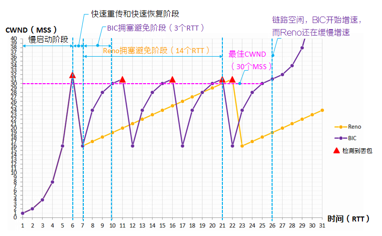
As shown in Figure 6, assuming the current network can transmit up to 30 MSS, the processing mechanisms of the Reno and BIC algorithms are as follows:

1.     Upon TCP connection establishment, it enters the slow start phase with the initial value of the congestion window CWND being 1 (MSS). The congestion window CWND gradually increases to 1, 2, 4, 8, 16, 32, following exponential growth. Reno and BIC processing are the same.

2.     The transmitter sends packets with a congestion window CWND 32, and network congestion occurs (the current network can transmit a maximum of 30 MSS). Upon receiving three duplicate ACK messages, the transmitter immediately retransmits the failed message section. Reno and BIC processing is the same.

3.     The transmitting end performs a fast restoration, reducing both the slow start threshold (ssthresh) and the congestion window to 32/2=16 MSS. Both Reno and BIC handle this in the same way.

4.     The transmitter enters the congestion avoidance stage and gradually increases the congestion window CWND. The processing of Reno and BIC varies.

¡     The congestion window of Reno increased from 16 to 30, requiring 14 RTTs.

¡     The congestion window of BIC increases from 16 to 30, requiring 3 RTTs (saving 11 RTTs compared to Reno). The 3 sniffer points corresponding to the CWND are 24 (16+8), 28 (16+8+4), and 30 (16+8+4+2).

From this, it is evident that when the link is free, BIC can quickly utilize the bandwidth, demonstrating a significantly higher preemption ability than Reno.

Figure 6 Schematic Diagram of the Principles of Reno and BIC Algorithms

 

Summary of Reno and BIC algorithms

When the network bandwidth increases, or the RTT gets larger, the advantages of BIC over Reno are more obvious. Therefore, BIC is better suited for communication networks than Reno. Upon its release, BIC immediately replaced Reno as the default congestion control algorithm for Linux.

Based on the principles of Reno and BIC, we can find that both Reno and BIC have the following usage constraints:

·     The algorithm misinterprets the error packages and random package losses generated during the transmission process as congestion losses. This significantly reduces the congestion window, lowers the transmit rate (Tx), and wastes network bandwidth.

·     To maximize the use of bandwidth, Reno and BIC will continue to increase the congestion window CWND as long as there are no lost packages, and they will try their best to transmit packages. This could cause a burst of packages, increasing the risk of packet loss. On the other hand, it could result in the accumulation of packages in the receive buffer of network devices that are not processed in time, thus increasing the transmission delay.

BBR

Concepts

Bottleneck bandwidth (BtlBw)

Bottleneck bandwidth refers to the maximum transmission capability of a transmission link. BBR (Bottleneck Bandwidth and RTT, or bottleneck bandwidth and round-trip delay) uses the bottleneck bandwidth BtlBw to control the number of packets that can be transmitted and the transmission rate from the transmitter. The transmitting end uses the packet arrival rate (i.e., the number of packets arrived in a section of time / the corresponding time interval) to calculate the instant bandwidth, and then estimates the bottleneck bandwidth BtlBw based on the instant bandwidth and the Kathleen Nichols algorithm.

RTprop (Round-Trip Time Delay Minimum Value)

RTprop refers to the minimum round-trip delay (RTT) time required for a package in the link to travel back and forth without queuing or loss.

Gain coefficient

BBR defines two gain coefficients:

·     The pacing_gain represents the adjustment multiplier of the transmission rate.

·     The cwnd_gain represents the adjustment factor of the transmit window.

The BBR algorithm defines four state machines: StartUp, Drain, ProbeBW (BtlBw detection phase), and ProbeRTT (RTprop detection phase). It assigns different gain coefficients for each state machine, adjusting the number of messages in the network by tuning these coefficients, for better sensing of changes in bandwidth and RTT.

·     During the StartUp phase, 'pacing_gain' is set to 2.89 and 'cwnd_gain' is also set to 2.89.

·     During the Drain section, the pacing_gain is set to 0.35 and the cwnd_gain is set to 2.89.

·     ProbeBW Stage: The ProbeBW stage is divided into 8 sub-sections. Within these 8 sections, the values of pacing_gain are 5/4, 3/4, 1, 1, 1, 1, 1, and 1, while the value of cwnd_gain is 2.

·     During the ProbeRTT phase, the value of pacing_gain is 1, and the value of cwnd_gain is also 1.

Principle of BBR algorithm

The BBR algorithm actively adjusts the congestion window and transmission rate based on measured feedback, thereby improving bandwidth utilization and preventing network congestion. BBR primarily uses the transmission rate to control the speed at which the transmitter sends packets, thus avoiding too fast transmission that may result in the receiving device not being able to process packets in time, leading to packet backlog. BBR also utilizes the congestion window to control the total amount of packets transmitted by the sending end, in order to prevent excessive packet transmission that could lead to network congestion.

The basic principle of the BBR algorithm is:

·     The transmitting end continuously measures the round-trip time delay (RTT) based on the transmitted section of the message and the ACK feedback received, and calculates the immediate network bandwidth (BW). The current immediate bandwidth (BW), round-trip time delay (RTT), historical bottleneck bandwidth (BtlBw, with an initial value of 0), and the historical minimum round-trip time delay (RTprop, with a larger initial value, being a 64-bit hexadecimal number f) are compared. Using the Kathleen Nichols algorithm, the current bottleneck bandwidth (BtlBw) and the current minimum round-trip time delay (RTprop) are determined.

·     BBR uses the obtained bottleneck bandwidth (BtlBw) and minimum RTT (RTprop), multiplied by the transmission rate gain coefficient (pacing_gain) and transmission window gain coefficient (cwnd_gain), to calculate the next congestion window and packet transmission rate.

¡     The actual packet dispatch rate, pacing_rate, is calculated by multiplying pacing_gain with BtlBw.

¡     The congestion window is calculated as the maximum value between the product of cwnd_gain, BtlBw, RTprop, and the constant number 4.

·     After BBR finds the bottleneck bandwidth (BtlBw) and the minimum RTT (RTProp), it mostly uses the BtlBw as the actual package transmission rate for steady transmissions. Then, it slightly increases or decreases the actual packet sending rate to detect new BtlBw and RTprop, in order to adapt to changes in the network environment.

Implementation process of BBR

BBR alternates through the following four states to conduct round-robin sniffing, in order to obtain BtlBw and RTprop: StartUp (Startup phase), Drain (Drain phase), ProbeBW (BtlBw sniffer phase), ProbeRTT (RTprop sniffer phase).

 

NOTE: In order to obtain the bottleneck bandwidth (BtlBw), BBR would increase the packet sending quantities, which may result in packet caching in the link queue, leading to an increase in round-trip time delay (RTT). To measure the minimum value of RTT (RTprop), the current link queue's cache needs to be cleared. Therefore, the simultaneous detection of BtlBw and RTprop is not feasible and requires alternating round-robin detection of BtlBw and RTprop.

 

StartUP (Startup phase)

After the TCP connection establishment, the BBR algorithm is activated and enters the StartUP state. The StartUP state corresponds to the launch phase of the BBR algorithm, aiming to obtain the current bottleneck bandwidth, BtlBw.

In order to detect the best packet sending rate quickly, under the StartUP state, BBR prescribes the packet sending gain coefficient (pacing_gain) as 2.89, and the current packet sending rate is pacing_gain*BtlBw=2.89*BtlBw.

The process for BBR's bottleneck bandwidth (BtlBw) detection is as follows:

1.     Initially, the transmitter sends messages to the receiver at a lower packet transmission rate to obtain the current real-time bandwidth (BW). If the BW is greater than the current bottleneck bandwidth (BtlBw, with an initial value of 0), it updates the bottleneck bandwidth and sets BtlBw equal to the real-time bandwidth (BW).

2.     Update the transmission rate, the current transmission rate = pacing_gain * BtlBw = 2.89 * BtlBw. The transmitter sends packets at a higher release rate.

3.     BBR continues to update the bottleneck bandwidth (BtlBw), using the new BtlBw to calculate the new transmission rate (RT). Then, it transmits the packets at this new rate.

4.     If BBR, after 3 consecutive sniffer calculations, finds that the instant bandwidth (BW) is consistently less than 1.25 times the current bottleneck bandwidth (BtlBw), it means BtlBw has been reached and package buffering may be occurring in the link. BBR will then transition into the Drain state.

Drain state

During the StartUP state, BBR increases the package sending rate at 2.89 times the speed. With the continuous growth of the package sending rate, package caching may occur in the link (network transmission equipment and receiver store messages that can't be processed in time in the receive buffer). Package caching means messages can't be processed immediately upon arrival at the receiving device. This can increase the round-trip time (RTT), and as more and more messages get cached, the receive buffer of the receiving device may become full, causing messages to be discarded. TCP needs to retransmit messages, leading to a sharp deterioration in transmission performance.

BBR aims to utilize the bandwidth at its maximum capacity, sending packages at the bottleneck bandwidth BtlBw. Also, the link should ideally be free from package buffers, to ensure that the messages can be delivered to the receiving end as quickly and swiftly as possible. Hence, after the StartUP state, BBR will enter the Drain state to purge the messages buffered in the link during the StartUP state.

The process of draining cached messages in BBR link is as follows:

1.     In order to clear the cached messages in the link, BBR needs to reduce the package sending rate. In the Drain state, the protocol stipulates that the package sending gain coefficient 'pacing_gain' is 0.35, and the package sending rate is 'pacing_gain * BtlBw = 0.35 * BtlBw.

2.     BBR sends packages at a rate of 0.35*BtlBw until it detects the number of messages being transmitted in the link is less than BtlBw*RTprop. At this time, BBR believes that the messages cached in the link queue have been emptied, and it enters the ProbeBW state.

ProbeBW state (during the BtlBw sniffer section)

Upon detecting the bottleneck bandwidth BtlBw and clearing cached packets in the link, BBR enters the ProbeBW state. During this phase, BBR mainly sends packets at a steady rate based on the bottleneck bandwidth BtlBw for most of the time, while slightly adjusting the packet sending rate occasionally to detect the new bottleneck bandwidth BtlBw.

Most of the time, BBR is in the ProbeBW state. This state consists of a round-robin cycle with a period of 8 RTTs, including 6 steady periods, 1 rising period, and 1 decreasing period.

·     6 stable periods: To fully utilize the network bandwidth, BBR sends packages steadily within 6 RTTs. At this time, the package sending gain coefficient pacing_gain=1, and the package sending rate=pacing_gain*BtlBw=1*BtlBw.

·     One rising period: To sniff a higher BtlBw, BBR briefly increases the package sending rate within one RTT. At this time, the package sending gain coefficient, pacing_gain, equals 1.25 and the package sending rate equals pacing_gain * BtlBw, which is 1.25 * BtlBw.

·     Decrease period for one RTT: In order to empty the cached messages in the link queue, BBR briefly reduces the package sending rate within one RTT. At this time, the sending gain coefficient (pacing_gain) is 0.75, and the sending rate (RT) is pacing_gain*BtlBw = 0.75*BtlBw.

ProbeRTT state (RTprop sniffer section)

RTprop refers to the minimum duration required for a package to travel back and forth in a link, i.e., the smallest round-trip time (RTT), assuming no queuing or packet loss in the link. Usually, RTprop becomes a fixed value after the link is established. However, since the transmission network is shared, there may be no messages transmitted by this connection in the link, but messages from other sessions may exist. Therefore, to ensure the reliability of the RTprop value, BBR checks the refresh state of the RTprop value. If RTprop hasn't been updated for more than 10 seconds, regardless of whether BBR is currently in StartUP, Drain, or ProbeBW state, it enters the RTprop state.

After entering the RTprop state, BBR reduces the congestion window to 4 and maintains this for 200 milliseconds (ms), clearing cached messages in the link by drastically reducing the packet sending. This facilitates the sniffer to detect the new RTprop.

BBR algorithm summary

Compared to Reno and BIC, the main advantages of BBR are demonstrated in the following aspects:

·     BBR adjusts the congestion window based on period sniffer results, not using packet loss as a trigger condition for congestion control, which is more reasonable and efficient than Reno and BIC.

·     Reno and BIC use the congestion window control to transmit packages, which inevitably leads to messages in the link being queued, increasing the transmission delay in the network. The larger the queue, the more severe the delay. BBR uses both the sending rate and the congestion window as parameters to control package transmission, enabling smooth delivery of burst messages. Moreover, BBR periodically slows down the transmission rate, clearing queued messages in the link, effectively reducing network delay.

·     BBR sends packages steadily most of the time, while Reno and BIC require round robin sniffer, package loss, quick restoration, and sniffer. The bandwidth utilization of BBR is higher and it has a greater throughput.

Of course, there are constraints to using BBR: given its cyclical nature, as well as the increase limit (1.25* BtlBw) for the period of ProbeBW state and decrease limit (0.75* BtlBw) for the period, BBR's preemption capability is less than BIC when network bandwidth increases or decreases. BIC responds quickly. If most connections in the link are short-duration TCP connections, the transmission efficiency of using BIC is higher.

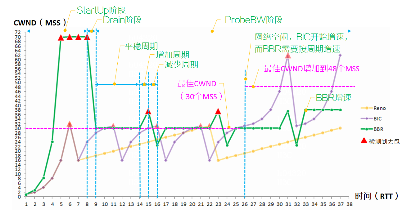
As shown in Figure 7, after the StartUp and Drain phases, BBR enters a relatively stable packet dispatching phase, where its throughput in the same time period is greater than that of Reno and BIC. When the network transmission capacity increases, the optimal congestion window increases from 30 MSS to 48 MSS. BIC only requires at least 5 RTTs to reach the optimal congestion window. However, BBR needs 7 RTTs for the congestion window to rise to 37 (1.25*30=37.5, taking 37 MSS). After another 8 RTTs, BBR's congestion window rises to 46 (1.25*37=46.25, taking 46 MSS).

Figure 7 Schematic diagram of the principles of Reno, BIC, and BBR algorithms

 

Introduction to BBRv2

The implementation of the standard BBR is called BBRv1. To compensate for the usage constraints of BBRv1 in a network coexisting with multiple algorithms (BBR, BIC algorithm) in terms of bandwidth preemption capabilities, BBRv2 was derived from BBR. BBRv2 is an optimization of BBRv1, the aspects of optimization include but are not limited to:

·     In the Startup state, BBRv2 has added a packet loss exit condition. To avoid more severe packet loss, it exits the Startup state as soon as packet loss is detected, without having to wait for "the immediate bandwidth BW calculated by continuous three-time sniffer to be less than 1.25 times the current bottleneck bandwidth BtlBw".

·     In order to respond quickly to network changes, TCP needs to timely adjust the congestion window CWND. Rapid adjustment of the CWND value can be achieved by speeding up the update of ProbeRTT. BBRv2 reduces the trigger condition for entering RTprop state from 10 seconds to 2.5 seconds. That is, if the RTprop has not been updated for a continuous 2.5 seconds, BBRv2 will immediately enter the ProbeRTT state to sniff the new RTprop.

·     To reduce the bandwidth fluctuation caused by entering the ProbeRTT state, once entered the ProbeRTT state, BBRv2 reduces the congestion window CWND to 0.5*BtlBw*RTprop, while BBRv1 reduces the congestion window CWND to 4.

Comparison of congestion control algorithms

Reno and BIC control the number of packets that can be sent from the sender through the congestion window, whereas BBR controls the rate and volume of packets sent from the sender through the network's maximum bandwidth (BtlBw) and RTprop (minimum RTT). Their biggest difference lies in their unique mechanisms of detecting maximum link bandwidth. Overall, the trend is as follows:

·     Convergence speed (from fast to slow): BBR > BIC > Reno.

·     In terms of fairness (the ability of preemption in a deep cache scenario, from strong to weak), the ranking is: BIC > BBR > Reno.

·     Packet loss resistance capabilities (from strongest to weakest): BBR > BIC > Reno.

·     Network queuing delay (from low to high): BBR<Reno<BIC.

 

NOTE: Deep caching refers to a relatively large cache in the link, such as the receive (Rx) cache, queue in the intermediate equipment, and so on.

 

The key technology of each algorithm and recommended usage scenarios are shown as depicted in Table 1.

Table 1 Comparing Reno, BIC, and BBR Congestion Control Algorithms

Algorithm	Critical Technical	Scenarios
Reno	·     Triggering congestion control based on package loss, without distinguishing whether the loss is due to erroneous packages or actual network congestion, can easily lead to a misjudgment. ·     When packet loss is detected, the congestion window is halved. ·     Linearly increase the congestion window using a sniffer; after every Round-Trip Time (RTT), add 1 to the congestion window.	For scenarios that require low packet loss rate, low bandwidth, and low latency requirements.
BIC	·     Using package loss as the trigger condition for congestion control without distinguishing between erroneous packages and actual network congestion can easily lead to misjudgment. ·     When packet loss is detected, the congestion window is halved. ·     Use binary search and multiplicative increase methods to sniff the congestion window CWND.	Scenarios requiring low packet loss rates, high bandwidth, and low latency requirements.
BBRv1	Instead of using package loss as a trigger condition for congestion control, calculate the congestion window and transmission rate based on the period sniffer delay and bandwidth, and transmit packages smoothly.	There is a scenario where there is a certain packet loss rate, high bandwidth, high demand for time delay, and the BBR algorithm is used independently.
BBRv2	Compared to BBRv1: ·     When BBRv2 is in the Startup state, it will exit the Startup state as soon as it detects packet loss, in order to prevent more severe packet loss. ·     The trigger condition for BBRv2 to enter the RTprop state is reduced from 10 seconds to 2.5 seconds (if RTprop has not been updated for a continuous 2.5 seconds, BBRv2 immediately enters the ProbeRTT state to sniff out the new RTprop). This allows for the timely adjustment of the congestion window and to promptly respond to network changes. ·     After entering the ProbeRTT state, BBRv2 reduces the congestion window to 0.5*BtlBw*RTprop to decrease the bandwidth fluctuation caused by the ProbeRTT state entry (BBRv1 reduces the CWND to 4).	There is a scenario where packet loss rate is present, the bandwidth is high, the requirement for time delay is high, and various algorithms coexist.