H3C Data Center Network Solution Underlay Network Design Guide

 

 

 

 

 

 

 

 

 

 

 

 

 

 

 

 

 

 

 

 

 

 

 

 

 

 

 

 

 

 

 

 

 

 

 

Document version: 6W100-20221206

 

Contents

Overview·· 1

Solution architecture· 1

Features· 1

Network design principles· 1

Leaf gateway design· 2

Routing protocol selection· 5

Capacity planning· 8

Multi-fabric expansion· 10

Recommended hardware· 12

Access design· 12

Server access design· 12

Connecting border devices to external gateways· 14

M-LAG topology· 14

Triangle topology· 15

Square topology· 16

IP planning principles· 17

Deployment modes· 17

About the deployment modes· 17

Management network configuration· 18

 

Overview

A data center network interconnects servers in a data center, distributed data centers, and data center and end users. Data center underlay connectivity protocols have gradually evolved from primarily Layer 2 protocols to primarily IP routing protocols. Driven by the scale of computing, the physical topology of data centers has evolved from an access-aggregation-core three-tier network architecture to a CLOS-based two-tier spine-leaf architecture.

This document describes the underlay network that uses the spine-leaf architecture.

Solution architecture

The underlay network uses OSPF or EBGP for communication between servers or between servers and the external network, and uses M-LAG between leaf nodes for access reliability.

Select appropriate switch models and configure spine and leaf nodes as needed based on the access server quantity, interface bandwidth and type, and convergence ratio to build a tiered DC network for elastic scalability and service deployment agility.

Features

A typical data center fabric network offers the following features:

·     Support for one or multiple spine-leaf networks.

·     Flexible configuration and elastic scaling of spine and leaf nodes.

·     VLAN deployment for isolation at Layer 2, and VPN deployment for isolation at Layer 3.

As a best practice, use the following network models in a spine-leaf network:

·     Configure M-LAG for leaf nodes for access availability.

·     Interconnect leaf and spine devices at Layer 3, and configure OSPF or EBGP for equal-cost multi-path load balancing and link backup.

Network design principles

As a best practice, deploy S68xx switch series, S98xx switch series, and S12500 switch series in the data center, and configure spine and leaf nodes based on the network scale.

Figure 1 Spine-leaf architecture

 

Spine design

Use Layer 3 Ethernet interfaces to interconnect spine and leaf nodes to build an all-IP fabric.

Leaf design

·     Configure M-LAG, S-MLAG, or IRF on the leaf nodes to enhance availability and avoid single points of failure. As a best practice, configure M-LAG on the leaf nodes.

·     Connect each leaf node to all spine nodes to build a full mesh mode network.

·     Leaf nodes are typically Top of Rack (ToR) devices. As a best practice to decrease deployment complexity, use the controller to deploy configuration automatically or use zero-touch provisioning (ZTP) for deployment.

ZTP automates loading of system software, configuration files, and patch files when devices with factory default configuration or empty configuration start up.

Leaf gateway design

Gateway deployment scheme overview

As a best practice, configure M-LAG in conjunction with VLAN or VRRP on leaf nodes to provide redundant gateways for servers.

Table 1 Gateway deployment scheme

Gateway type	Description
Dual-active VLAN interfaces (recommended)	·     A VLAN interface is configured on each M-LAG member device, and both M-LAG member devices can respond to ARP packets and perform Layer 3 forwarding. ·     Attached servers require Layer 3 connectivity to the M-LAG system in some scenarios, K8s containers are deployed on the servers for example. To fulfil this requirement, perform one of the following tasks: ¡     Configure static routes. ¡     Assign a virtual IPv4 or IPv6 address to each gateway VLAN interface by using the port m-lag virtual-ip or port m-la ipv6 virtual-ip command.
VRRP group	·     Both the VRRP master and backup devices perform Layer 3 forwarding, but only the master device responds to ARP packets. ·     The server-side devices can set up dynamic routing neighbor relationships with the M-LAG member devices.

 

M-LAG + dual-active VLAN interfaces

Configure a VLAN interface on each M-LAG member device, as shown in Figure 2. Both M-LAG member devices can respond to ARP packets and perform Layer 3 forwarding.

Figure 2 Network diagram

 

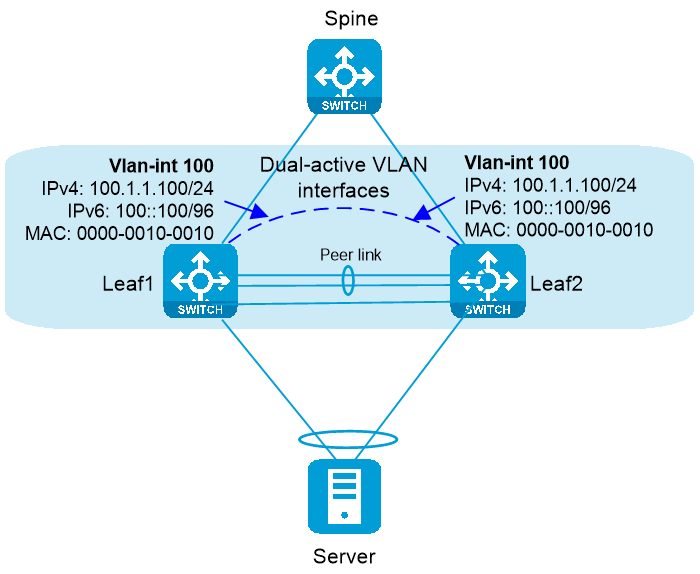
To configure dual-active VLAN interfaces on the M-LAG system, perform the following tasks:

1.     Create a gateway VLAN interface on each M-LAG member device for the same VLAN.

2.     Assign the same IPv4 and IPv6 addresses and MAC address to the gateway VLAN interfaces.

The dual-active VLAN interfaces operate as follows:

·     Each M-LAG member device forwards traffic locally instead of forwarding traffic towards the M-LAG peer over the peer link. For example, Leaf 1 will directly respond to an ARP request received from the server.

·     When one uplink fails, traffic is switched to the other uplink. For example, when Leaf 1 is disconnected from the spine device, traffic is forwarded as follows.

¡     Downlink traffic is switched to Leaf 2 for forwarding.

¡     When receiving uplink traffic destined for the spine device, Leaf 2 forwards the traffic locally. When Leaf 1 receives uplink traffic, it sends the traffic to Leaf 2 over the peer link, and Leaf 2 forwards the traffic to the spine device.

·     Traffic is load shared between the access links to increase bandwidth utilization.

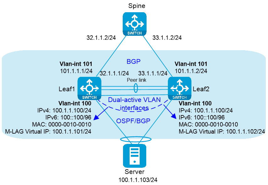
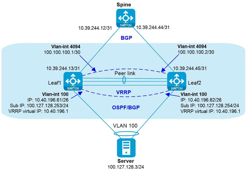
The dual-active VLAN interfaces use the same IP address and MAC address. As shown in Figure 3 and Table 2, for the M-LAG member devices to set up routing neighbor relationships with the server-side network device, perform the following tasks:

·     Use the port m-lag virtual-ip or port m-lag ipv6 virtual-ip command to assign an M-LAG virtual IP address to the dual-active VLAN interfaces.

·     Configure routing protocols.

The dual-active VLAN interfaces will use the virtual IP addresses to establish routing neighbor relationships.

Figure 3 Routing neighbor relationship setup

 

Table 2 Configuration tasks

Tasks

Forwarding

·     Dual-active VLAN interface configuration: a.     Create a VLAN interface on each M-LAG member device for the same VLAN. b.     Assign the same IP address and MAC address to the VLAN interfaces. c.     Assign a unique virtual IP address from the same subnet to each of the VLAN interfaces with the same VLAN ID. The VLAN interfaces use the virtual IP addresses for BGP or OSPF neighbor relationship setup. ·     Create a VLAN interface on each M-LAG member device for another VLAN, assign the peer-link interfaces to this VLAN, and assign a unique IP address from the same subnet to each of the VLAN interfaces. The M-LAG member devices use these VLAN interfaces to forward Layer 3 traffic between them when a link to the upstream spine device is failed. ·     Use Layer 3 interfaces to connect the M-LAG member devices to the upstream spine device, and configure ECMP routes for load sharing between the uplinks.

The traffic sent to the M-LAG system is load shared between the uplinks or downlinks. The M-LAG member devices forward traffic as follows: ·     For Layer 2 traffic sent by the server, the M-LAG member devices look up the MAC address table and forward the traffic locally. ·     For Layer 3 traffic sent by the server, the M-LAG member devices perform Layer 3 forwarding based on the FIB table. ·     For external traffic destined for the server, the M-LAG member devices perform forwarding based on the FIB table.

 

M-LAG + VRRP gateways

You can configure VRRP groups on an M-LAG system to provide gateway services for the attached server, as shown in Figure 4 and Table 3.

Figure 4 Network diagram

 

Table 3 Configuration tasks

Tasks

Forwarding

·     Configure a VRRP group on the M-LAG member devices and use the VRRP virtual IP address as the gateway for the attached server. ·     VLAN interface configuration: a.     Create a VLAN interface for the VLAN where the M-LAG interface resides on each M-LAG member device. b.     Assign a unique primary IP address from the same subnet to each of the VLAN interfaces. c.     Assign a unique secondary IP address from another subnet to each of the VLAN interfaces. ·     Use the primary or secondary IP addresses of the VLAN interfaces to set up BGP or OSPF neighbor relationships with the server-side network device. ·     Set up a Layer 3 connection over the peer link between the M-LAG member devices. The M-LAG member devices use the Layer 3 connection to forward traffic between them when a link to the upstream spine device is failed. ·     Use Layer 3 interfaces to connect the M-LAG member devices to the upstream spine device, and configure ECMP routes for load sharing between the uplinks.

The traffic sent to the M-LAG system is load shared between the uplinks or downlinks. The M-LAG member devices forward traffic as follows: ·     For the Layer 3 traffic sent by the server, both M-LAG member devices perform Layer 3 forwarding. ·     For the external traffic destined for the server, the M-LAG member devices make forwarding decisions based on local routes.

 

Routing protocol selection

About underlay routing protocol selection

As a best practice, select OSPF or EBGP as the underlay routing protocol based on the network scale.

Table 4 About underlay routing protocol selection

Protocol	Advantages	Disadvantages	Applicable scenarios
OSPF	l     Simple deployment. l     Fast convergence. l     Because OSPF packets in the underlay and BGP packets in the overlay are in different queues, the VPN instance and route entries are isolated, implementing fault isolation.	l     Limited OSPF routing domain. l     Relatively large fault domain.	l     Single area in small- and medium-sized networks, and multiple areas in large networks. l     Recommended number of neighbors: Less than 200.
EBGP	l     Independent routing domain per AS. Controllable fault domain. l     Flexible route control and flexible scalability. l     Applicable to large networks.	Complicated configuration.	l     Medium-sized and large networks. l     Recommended number of neighbors: Less than 500.

 

Detailed OSPF characteristics

·     Network scale

¡     Applicable to a wide scope, and supports various network scales.

¡     Easy deployment. As best practice, deploy OSPF to small-sized networks.

·     Area-based OSPF network partition

¡     In large OSPF routing domains, SPF route computations consume too many storage and CPU resources. To resolve these issues, OSPF splits an AS into multiple areas. Each area is identified by an area ID.

¡     Area-based network partition can reduce the LSDB size, memory consumption and CPU load, as well as network bandwidth usage because of less routing information transmitted between areas.

¡     For a single-fabric network, you can deploy internal devices to the same OSPF area.

¡     For a multi-fabric network, deploy each area to a different fabric, and connect the areas through the backbone area.

·     ECMP: Supports multiple equal-cost routes to the same destination.

·     Fast convergence: Advertises routing updates instantly upon network topology changes.

Detailed BGP characteristics

BGP is more advantageous in large networks with the following characteristics:

·     Reduces bandwidth consumption by advertising only incremental updates.

·     Reduces the number of routes by using route aggregation, route dampening, community attributes, and route reflection.

When more than 200 leaf nodes exist, as a best practice, use EBGP to deploy underlay network routes. For recommended deployment solutions, see "Recommended BGP deployment solution 1" and "Recommended BGP deployment solution 2."

Recommended BGP deployment solution 1

Figure 5 Recommended EBGP route planning within a single fabric

 

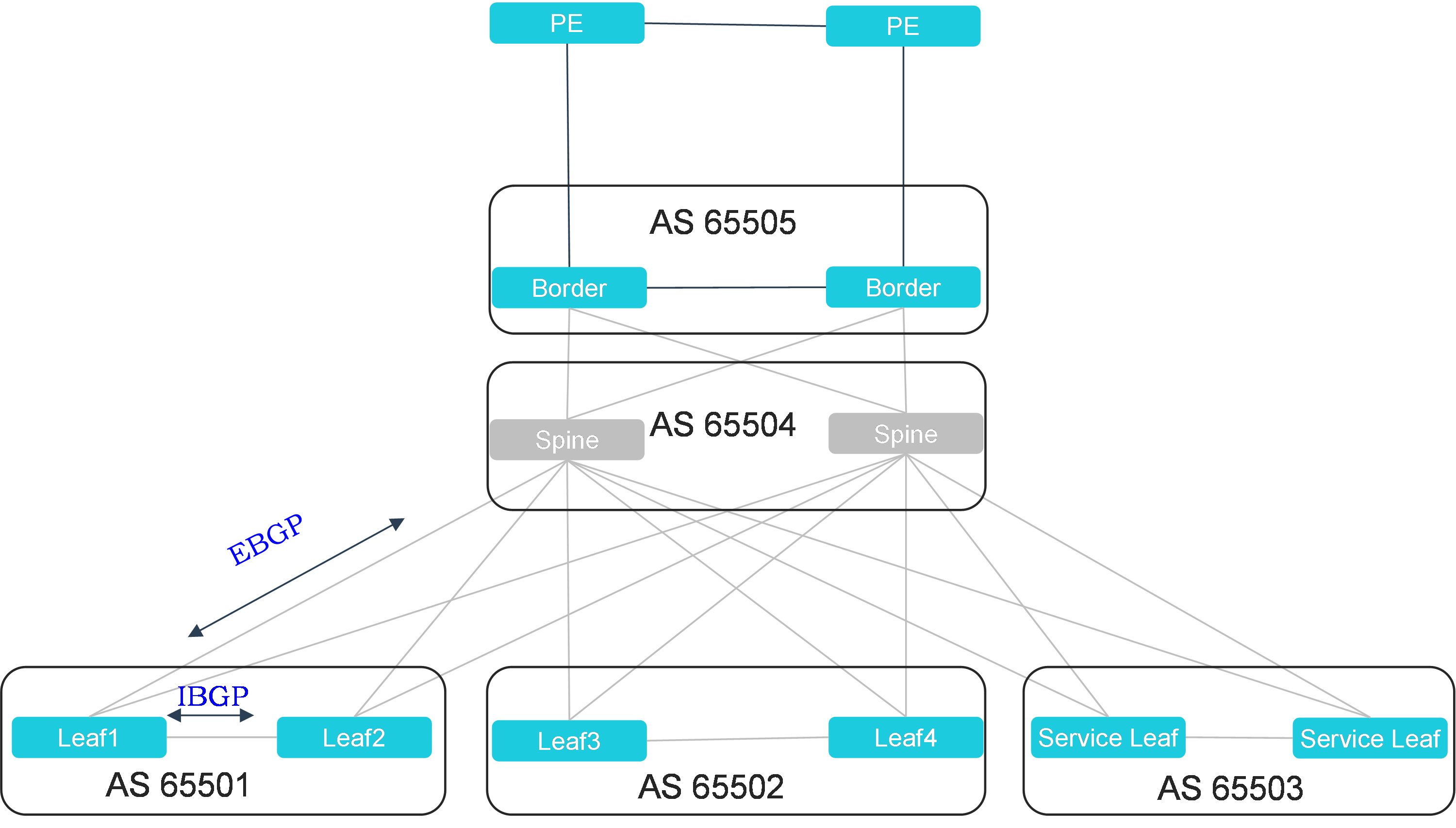
Characteristics of recommended BGP deployment solution 1:

·     Assign an AS number to each group of leaf devices, and you do not need to disable BGP routing loop prevention.

·     Establish IBGP peers between leaf devices in a group over the peer link, and establish EBGP peers between leaf devices and spine devices.

·     An uplink failure can trigger a switchover through the peer link. The current solution supports switchover by establishing neighbors through the peer link between the M-LAG devices. Switchover through Monitor Link will be added in the future as planned.

Recommended BGP deployment solution 2

Figure 6 Recommended EBGP route planning within a single fabric

 

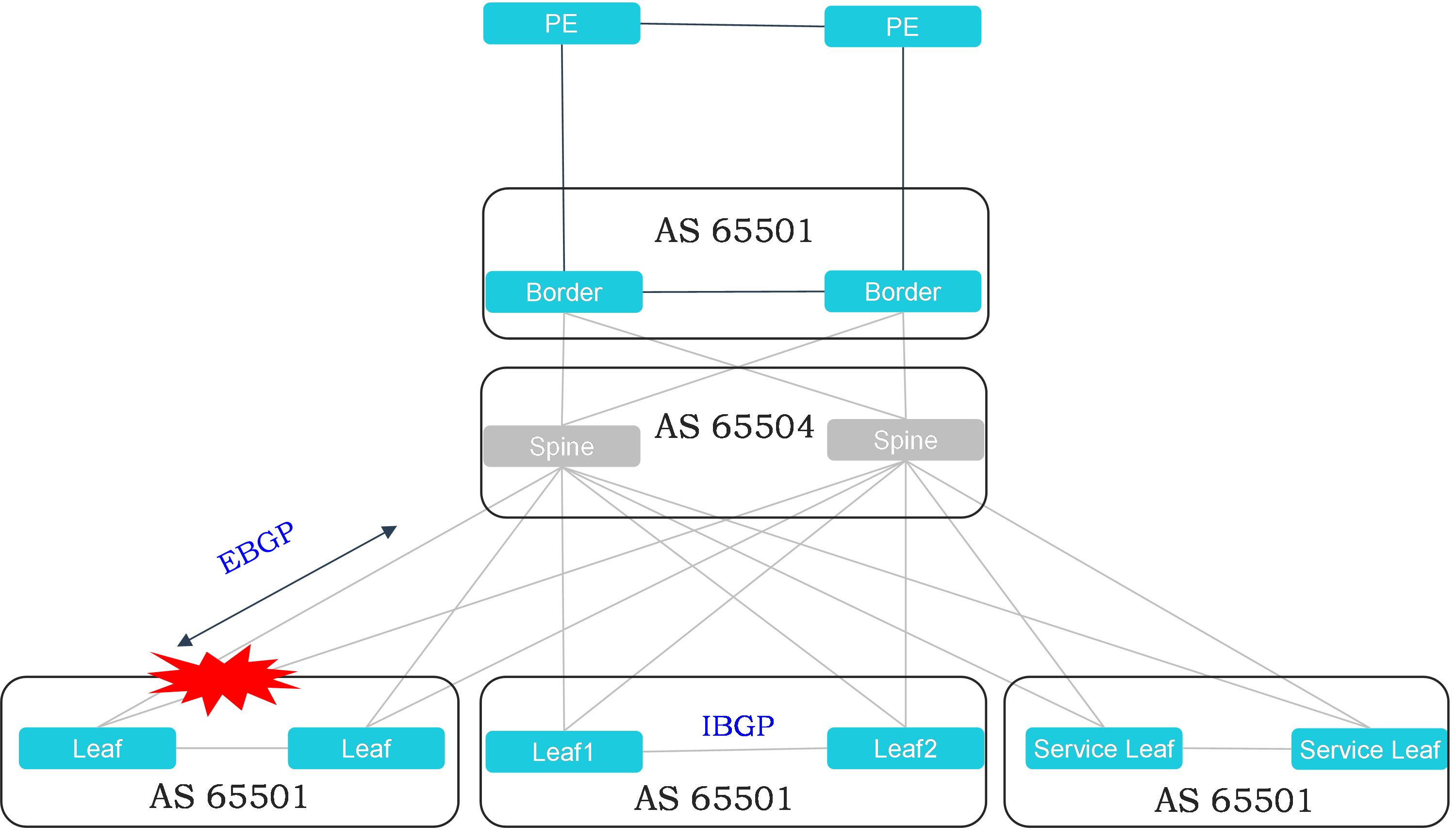
Characteristics of recommended BGP deployment solution 2:

·     Assign the same AS number to all leaf and border devices.

·     Establish EBGP peers between leaf or border devices in each group with the spine devices. Establish IBGP peers between the two devices in each group.

·     Because all leaf and border devices use the same AS number, you need to disable BGP routing loop prevention on leaf and border nodes. Alternatively, configure a routing policy on the spine nodes for AS-PATH replacement (recommended) as follows:

¡     route-policy AS_Replace permit node node-number

¡     apply as-path 65504 replace

¡     peer group-name route-policy AS_Replace import

·     The current solution supports switchover by establishing neighbors through the peer link between the M-LAG devices. Switchover through Monitor Link will be added in the future as planned.

Capacity planning

This section introduces the server capacity design within a single fabric.

Design principles

The number of spine downlink interfaces is the number of leaf devices. Number of servers = Number of leaf devices × number of leaf downlink interfaces / 2.

Typical design

·     M-LAG access

When the access switches adopt M-LAG, the leaf devices that form an M-LAG system use two high-speed ports to establish the peer link, and four ports in the uplink. Among the four ports, each two ports are connected to one spine device.

Table 5 The leaf devices adopt 10-G interfaces to connect to the servers and 40-G uplink interfaces

Spine device model	Number of spine devices	Spine convergence ratio (uplink/downlink)	Number of access switches	Number of access servers
S12516X-AF	2	Evaluation based on 36 × 40-G interface card: Convergence ratio (1:3) That is, 144 uplink ports and 432 downlink ports.	432 / 2 = 216 Convergence ratio (1:3) That is, 160:480 (4 × 40-G uplink ports and 48 × 10-G downlink ports per switch).	216 × 48 / 2 = 5184
		Evaluation based on 36 × 40-G interface card: Convergence ratio (1:1) That is, 288 uplink ports and 288 downlink ports.	288 / 2 = 144 Convergence ratio (1:3) That is, 160:480 (4 × 40-G uplink ports and 48 × 10-G downlink ports per switch).	144 × 48 / 2 = 3456

 

Table 6 The leaf devices adopt 25-G interfaces to connect to the servers and 100-G uplink interfaces

Spine device model	Number of spine devices	Spine convergence ratio (downlink/uplink)	Number of access switches	Number of access servers
S12516X-AF	2	Evaluation based on 36 × 100-G interface card: Convergence ratio (1:3) That is, 144 uplink ports and 432 downlink ports.	432 / 2 = 216 Convergence ratio (1:3) That is, 400:1200 (4 × 100-G uplink ports and 48 × 25-G downlink ports per switch).	216 × 48 / 2 = 5184
		Evaluation based on 36 × 100-G interface card: Convergence ratio (1:1) That is, 288 uplink ports and 288 downlink ports.	288 / 2 = 144 Convergence ratio (1:3) That is, 400:1200 (4 × 100-G uplink ports and 48 × 25-G downlink ports per switch).	144 × 48 / 2 = 3456

 

·     S-MLAG access

When the access switches adopt S-MLAG access, each access switch uses six or eight uplink ports. Each port corresponds to one spine device.

Table 7 The leaf devices use 10-G interfaces to connect to the servers and 100-G uplink interfaces

Spine device model	Number of spine devices	Spine convergence ratio (uplink/downlink)	Number of access switches	Number of access servers
S9820-8C	6	Convergence ratio (1:3) That is, 32 uplink ports and 96 downlink ports.	96 Convergence ratio (5:4) That is, 600:480 (6 × 100-G uplink ports and 48 × 10-G downlink ports per switch).	96 × 48 / 2 = 2304
		Convergence ratio (1:1) That is, 64 uplink ports and 64 downlink ports.	64 Convergence ratio (5:4) That is, 600:480 (6 × 100-G uplink ports and 48 × 10-G downlink ports per switch).	64 × 48 / 2 = 1536

 

Table 8 The leaf devices use 25-G interfaces to connect to the servers and 100-G uplink interfaces

Spine device model	Number of spine devices	Spine convergence ratio (uplink/downlink)	Number of access switches	Number of access servers
S9820-8C	8	Convergence ratio (1:3) That is, 32 uplink ports and 96 downlink ports.	96 Convergence ratio (2:3) That is, 800:1200 (8 × 100-G uplink ports and 48 × 25-G downlink ports per switch).	96 × 48 / 2 = 2304
		Convergence ratio (1:1) That is, 64 uplink ports and 64 downlink ports.	64 Convergence ratio (2:3) That is, 800:1200 (8 × 100-G uplink ports and 48 × 25-G downlink ports per switch).	64 × 48 / 2 = 1536

 

Multi-fabric expansion

You can add more fabrics to further expand the data center network. Connect the fabrics with EDs.

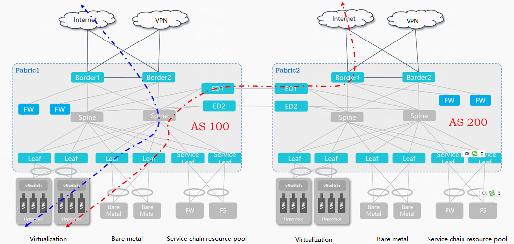
Figure 7 Single fabric network diagram

 

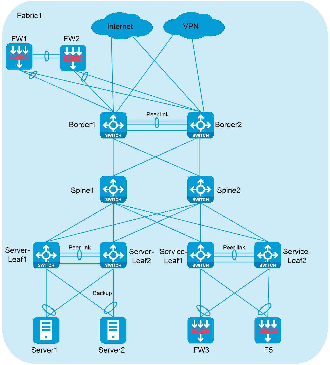
Figure 8 Multiple fabrics connected with EDs

 

Recommended hardware

Device role	Scenario	Device model
Border/ED	Medium-sized and large networks	·     Type H modules for the S12500X-AF switches ·     All modules supported by the S12500G-AF switches
	Small-sized networks	Same as the leaf devices
Spine	More than 3000 servers	Type H modules for the S12500X-AF switches
		All modules supported by the S12500G-AF switches
	1000 to 3000 servers	S9820-8C
	Less than 1000 servers	S68xx
Leaf	10-GE access	·     S6800 ·     S6860 ·     S6805 ·     S6850-2C/S9850-4C with 10-GE interface modules installed ·     S6812/S6813 ·     S6880-48X8C
	25-GE access	·     S6825 ·     S6850-56HF ·     S6850-2C/S9820-4C with 25-GE interface modules installed ·     S6880-48Y8C
	40-GE access	·     S6800 ·     S6850-2C/S9850-4C with 40-GE interface modules installed
	100-GE access	·     S9850-32H ·     S6850-2C/S9850-4C with 100-GE interface modules installed ·     S9820-8C ·     S9820-64H

 

Access design

Server access design

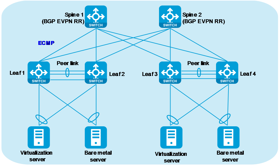
Every two access devices form an M-LAG system of leaf devices to provide redundant and backup access for servers.

Figure 9 Typical data center network

 

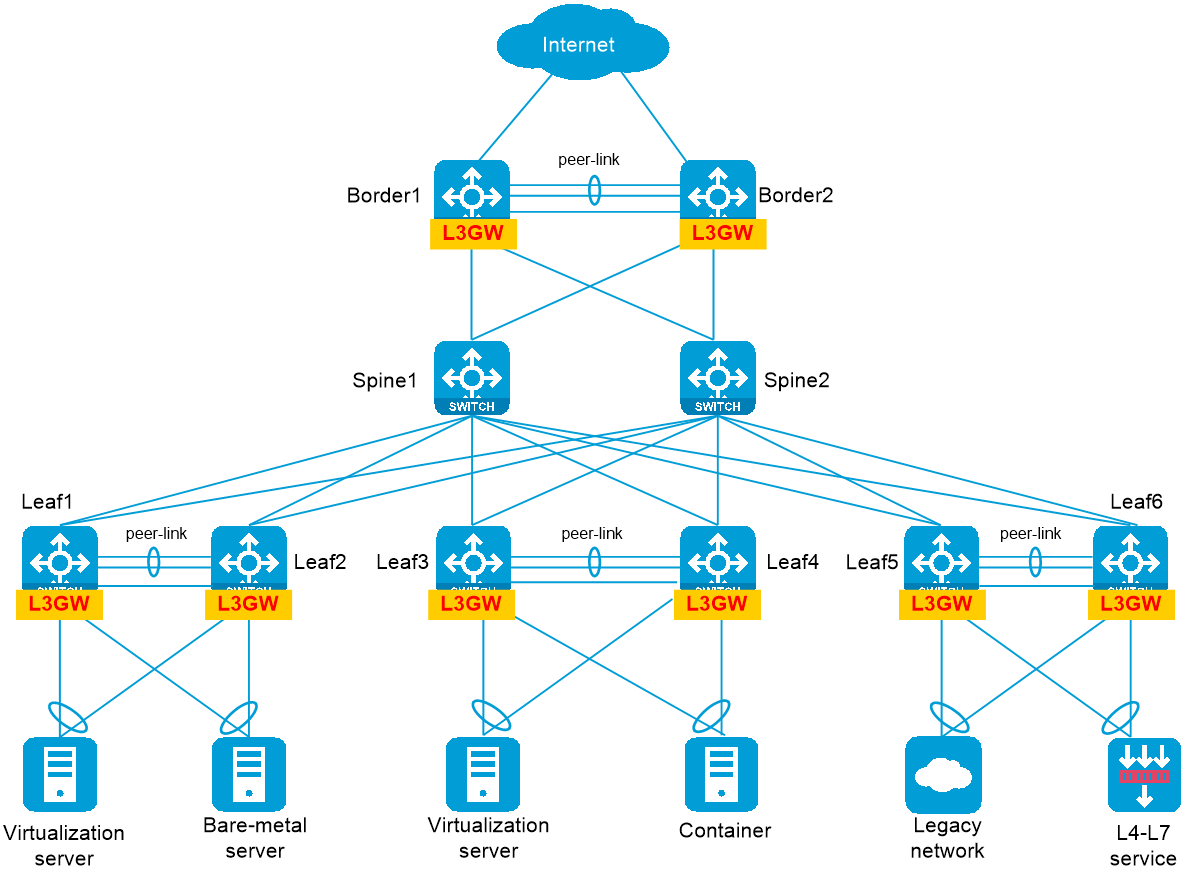
As a best practice, use one of the following server access solutions:

·     A server accesses an M-LAG system of leaf devices in primary/backup mode. Physical interfaces act as common trunk access interfaces, and are not assigned to the M-LAG group. When the primary link is operating normally, the backup link does not receive or send packets. When the primary link fails, a primary/backup link switchover occurs for the server, and ARP and ND entries are updated to trigger remote route updates.

·     A server accesses an M-LAG system of leaf devices in load sharing mode. An aggregate interface acts as a trunk access interface, and is assigned to the M-LAG group. Both links of the server operate at the same time.

Figure 10 Server access methods

 

Connecting border devices to external gateways

Border devices can be connected to external gateways by using the following methods:

·     M-LAG topology

·     Triangle topology

·     Square topology

M-LAG topology

Network topology

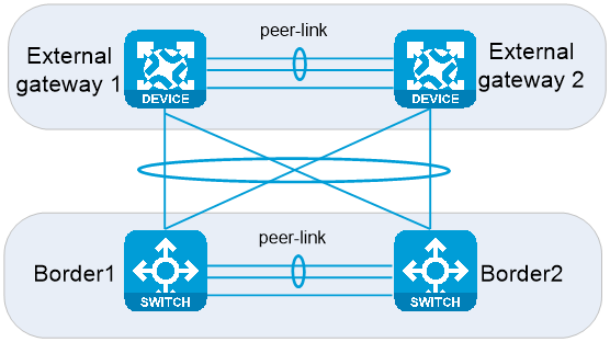
As shown in Figure 11, two border devices form an M-LAG system, and two external gateways also form an M-LAG system. The physical cables are cross-connected among border devices and external gateways. Four links among border devices and external gateways are aggregated to form a logical link through M-LAG. Because an external network specifies only one gateway IP for an external gateway and the M-LAG network requires only one interconnect IP for one aggregate link, this network topology is well compatible with the cloud network model. As a best practice, use the M-LAG network if possible.

Figure 11 M-LAG topology for border devices and external gateways

 

Reliability

On the M-LAG network, you do not need to deploy failover links between border devices. The traffic will not be interrupted only if one of the four physical links among the border devices and external gateways is normal.

·     When one link between Border1 and external gateways fails, LACP automatically excludes the faulty link and switches traffic to the normal link, which is transparent for routing.

·     When both links between Border1 and external gateways fail, M-LAG keeps the aggregate interface up, and the traffic is switched to Border2 over the peer link. Then, the traffic is forwarded to external gateways through the normal aggregate interface, which is transparent for routing.

·     When Border1 fails, the underlay routing protocol senses the failure. On the spine device, the routing protocol withdraws the route with the next hop VTEP IP as Border1, and switches to Border2 the traffic previously load-shared to Border1 in equal cost mode.

Benefits and restrictions

The external gateways must also support M-LAG. An M-LAG system supports only two member devices.

Fewer IP addresses and VLAN resources are consumed. The M-LAG topology is well compatible with the cloud network model.

Triangle topology

Network topology

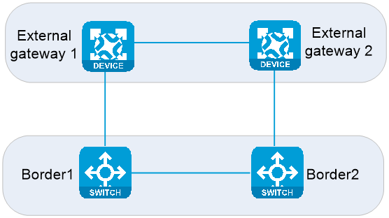
As shown in Figure 12, two border devices form a multi-active device group, which supports more than two devices. Border devices use four Layer 3 interfaces to connect to eternal gateways, and the physical cables are cross-connected. The border devices and external gateways can communicate through static routes and OSPF routes.

Figure 12 Triangle topology for border devices and external gateways

 

Reliability

In the triangle topology, failover links between Border1 and Border2 are not required. The failover links between border devices are needed only when all links between a border device and external gateways fail.

·     When one link between Border1 and external gateways fails, the corresponding static routes are invalidated or the corresponding dynamic routes are withdrawn. Then, the traffic previously load-shared to the faulty link in equal cost mode can be switched to the other normal link.

·     When both links between Border1 and external gateways fail, failover links are needed between border devices for the network to operate normally. In this case, the corresponding static routes are invalidated or the corresponding dynamic routes are withdrawn. Then, the traffic on Border1 can pass through the failover links to reach Border2, and then be forwarded to external gateways through Border2.

·     When Border1 fails, the underlay routing protocol senses the failure. On the spine device, the routing protocol withdraws the route with the next hop VTEP IP as Border1, and switches to Border2 the traffic previously load-shared to Border1 in equal cost mode. In this case, the corresponding static routes are invalidated or the corresponding dynamic routes are withdrawn on the external gateways. Then, the traffic in the north-to-south direction can be switched to Border2.

Benefits

Two or more border devices can be active. More IP addresses and VLAN resources are consumed.

Square topology

Network topology

As shown in Figure 13, border devices use two Layer 3 interfaces to connect to external gateways. You must deploy a failover link between the two border devices, and make sure the preference of a failover route is lower than that of a route for normal forwarding. Typically, dynamic routing protocols are deployed between two external gateways and two border devices to automatically generate routes for normal forwarding and failover routes.

Figure 13 Square topology for border devices and external gateways

 

Reliability

In the square topology, you must deploy a failover link between Border1 and Border2. When the interconnect link between a border device and external gateways fails, the failover link is required for service continuity.

·     When the interconnect link between Border1 and external gateways fails, the corresponding static routes are invalidated or the corresponding dynamic routes are withdrawn. Then, the traffic on Border1 can pass through the failover link to reach Border2, and then be forwarded to external gateways through Border2.

·     When Border1 fails, the underlay routing protocol senses the failure. On the spine device, the routing protocol withdraws the route with the next hop VTEP IP as Border1, and switches to Border2 the traffic previously load-shared to Border1 in equal cost mode. In this case, the corresponding static routes are invalidated or the corresponding dynamic routes are withdrawn on the external gateways. Then, the traffic in the north-to-south direction can be switched to Border2.

Benefits

The square topology reduces the number of links between border devices and external gateways. This topology is applicable when the border devices are far from the external gateways or hard to connect to external gateways.

IP planning principles

On a single-fabric network, you must plan the spine-leaf interconnect interface addresses and router ID addresses.

Spine-leaf interconnect interface IP addresses

As a best practice, configure the spine-leaf interconnect interfaces to borrow IP addresses from loopback interfaces. On a Layer 3 Ethernet interface, execute the ip address unnumbered interface LoopBack0 command to configure the interface to borrow an IP address from a loopback interface.

Router ID address planning on an M-LAG network

For a routing protocol, two member devices of an M-LAG system are standalone and must be configured with different router IDs. Please manually configure router IDs. If you do not do that, a device will automatically select a router ID, which might cause router ID conflicts. In an EVPN+M-LAG environment, as a best practice, configure the network as follows:

·     Two member devices in the same M-LAG system use loopback0 interface addresses as the local VTEP IP address and router ID of the M-LAG system, and cannot be configured with the same address.

·     Two member devices in the same M-LAG system use loopback1 interface addresses as the virtual VTEP address (configured by using the evpn m-lag group command) and must be configured with the same address.

Deployment modes

About the deployment modes

The underlay network contains spine and leaf nodes.

You can deploy the underlay network in the following modes:

·     Manual deployment

·     Automated deployment

Automated deployment can be implemented in the following ways:

·     Automatic configuration deployment by the controller. You configure templates on the controller and devices can be incorporated by the controller automatically when they start up with factory default configuration. No underlay device provisioning is required.

·     Automatic configuration (recommended in scenarios without a controller deployed)

a.     The administrator saves the software image files (including startup image files and patch packages) and configuration files for the device to an HTTP, TFTP, or FTP server. The software image files and configuration files for the device can be identified by the SN of the device.

b.     The device obtains the IP address of the TFTP server through DHCP at startup and then obtains the script for automatic configuration.

c.     The device runs the script and obtains device information (for example, SN) and matches the software image file and configuration file for the device.

d.     The device downloads the software image file and configuration file from the file server, and loads the image and deploys configuration automatically.

Output from a Python script for automatic configuration enables you to monitor the operations during execution of that script, facilitating fault location and troubleshooting.

With the automatic configuration feature, the device can automatically obtain a set of configuration settings at startup. This feature simplifies network configuration and maintenance.

Management network configuration

In a data center network, a management switch connects to the management network of each device.

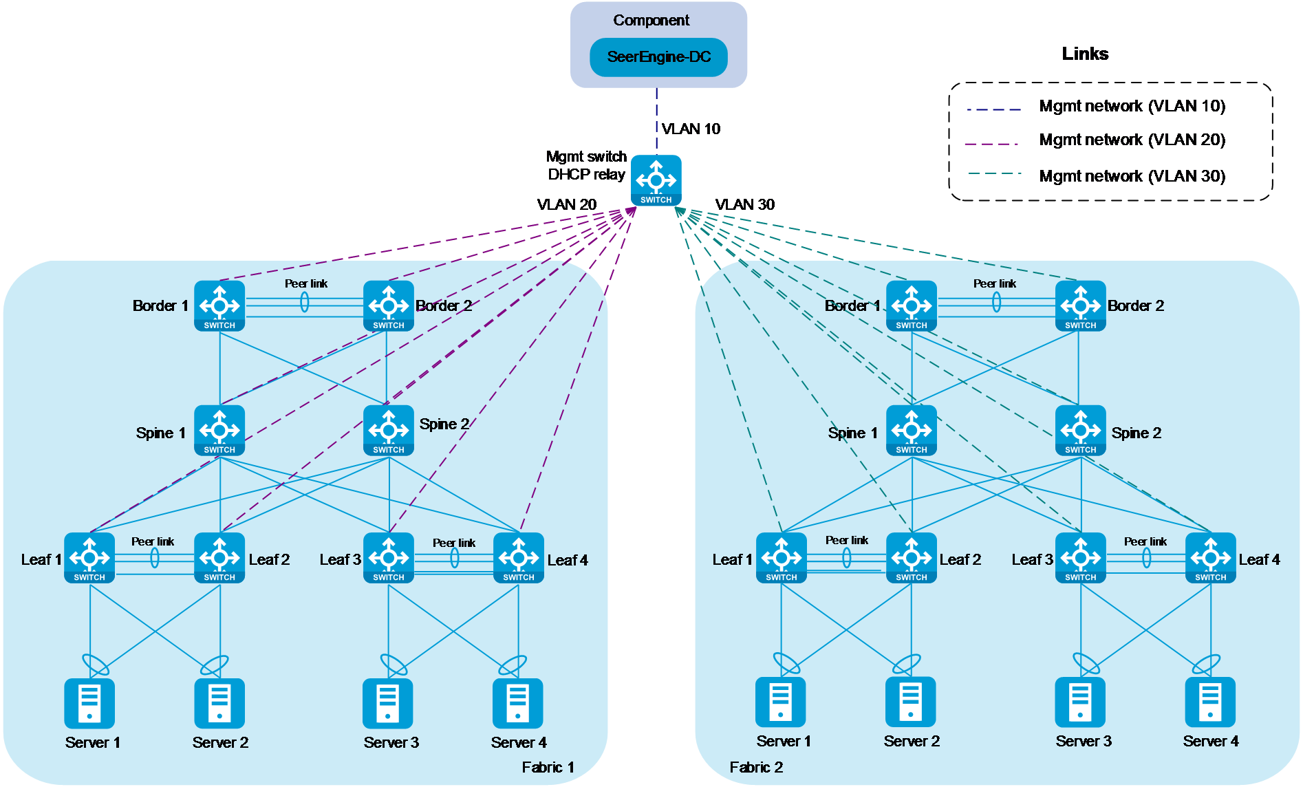
Use Layer 2 or Layer 3 networking mode for the management network in the single-fabric scenario. Use Layer 3 networking mode for the management network in the multi-fabric scenario. In Layer 3 networking mode, you must assign different VLANs to different fabrics, and manual configure a gateway and DHCP relay. As a best practice for future expansion of a fabric, use Layer 3 networking mode in the single-fabric scenario.

Figure 14 shows the management network in Layer 3 networking mode in the multi-fabric scenario.

Figure 14 Management network