- Released At: 12-05-2025
- Page Views:
- Downloads:
- Table of Contents
- Related Documents
-
|
|
|
QoS |
|
Technology White Paper |
|
|
|
|
Copyright © 2020 New H3C Technologies Co., Ltd. All rights reserved.
No part of this manual may be reproduced or transmitted in any form or by any means without prior written consent of New H3C Technologies Co., Ltd.
Except for the trademarks of New H3C Technologies Co., Ltd., any trademarks that may be mentioned in this document are the property of their respective owners.
This document provides generic technical information, some of which might not be applicable to your products.
The information in this document is subject to change without notice.
Contents
Introduction to QoS service models
Interoperability between IntServ and DiffServ
Traffic classification and marking
IPv4 QoS traffic classification
IPv6 QoS traffic classification
Ethernet QoS traffic classification
Congestion management technology comparison
Traditional packet drop policy
Relationship between WRED and queuing mechanism
Traffic shaping and traffic policing
QoS implementation in an enterprise VPN
Overview
Technical background
On traditional IP networks, devices treat all packets equally and handle them using the first in first out (FIFO) policy. All packets share the resources of the network and devices. A packet is assigned resources prior to all its subsequent packets. This service model is called best-effort. It delivers packets to their destinations as possibly as it can, providing no guarantee of delay, jitter, packet loss ratio, or reliability.
The Internet has been growing along with the fast development of networking technologies. Real-time applications, Voice over IP (VoIP) for example, require low transmission delay. Contrarily, E-mail and FTP applications are not sensitive to transmission delay. To satisfy different requirements of different services, such as voice, video, and data services, the network must identify these services and then provide differentiated services. As a traditional IP network in the best-effort service model does not identify services in the network, it cannot provide differentiated services.
The Quality of Service (QoS) technology was introduced to address this problem.
Benefits
The objective of QoS is to provide different levels of services for different services, for example:
· To limit FTP bandwidth in a backbone network and prioritize traffic accessing databases.
· To enable an Internet service provider (ISP) to identify voice, video, and other real-time traffic of its customers for differentiated service provisioning.
· To guarantee bandwidth and low delay for time-sensitive multi-media services, ensuring that they are not affected by the other services transmitted on the network.
Introduction to QoS service models
This section covers three typical QoS service models, each representing a set of end-to-end QoS capabilities. They are:
· Best-effort service
· Integrated service (IntServ)
· Differentiated service (DiffServ)
Best-effort service model
Best effort is a flat service model and also the simplest service model. In the best effort service model, an application can send packets without limitation, and does not need to request permission or inform the network in advance. The network delivers the packets at its best effort but does not provide guarantee of delay or reliability.
The best-effort service model is the default model in the Internet and is applicable to most network applications, such as FTP and E-mail. It is implemented through FIFO queuing.
IntServ service model
IntServ is a multiple services model that can accommodate various QoS requirements. In this model, an application must request a specific kind of service from the network before it can send data. The request is made by Resource Reservation Protocol (RSVP) signaling. RSVP signaling is out-of-band signaling. With RSVP, applications must signal their QoS requirements to network devices before they can send data packets.
An application first informs the network of its traffic parameters and QoS requirements for bandwidth, delay, and so on. When the network receives the QoS requirements from the application, it checks resource allocation status based on the QoS requirements and the available resources to determine whether to allocate resources to the application. If yes, the network maintains a state for each flow (identified by the source and destination IP addresses, source and destination port numbers, and protocol), and performs traffic classification, traffic policing, queuing, and scheduling based on that state. When the application receives the resource allocation acknowledgement from the network, the application starts to send packets. As long as the traffic of the application remains within the traffic specifications, the network commits to meeting the QoS requirements of the application.
IntServ provides two types of services:
· Guaranteed service, which provides assured bandwidth and limited delay. For example, you can reserve 10 Mbps of bandwidth and require delay less than 1 second for a Voice over IP (VoIP) application.
· Controlled load service, which guarantees some applications low delay and high priority when overload occurs to decrease the impact of overload on the applications to near zero.
DiffServ service model
DiffServ is a multiple services model that can satisfy diverse QoS requirements. Unlike IntServ, DiffServ does not require an application to signal the network to reserve resources before sending data, and therefore does not maintain a state for each flow. Instead, it determines the service to be provided for a packet based on the DSCP value in the IP header.
In a DiffServ network, each forwarding device performs a forwarding per-hop behavior (PHB) for a packet based on the Differentiated Services Code Point (DSCP) field in the packet. The forwarding PHBs include:
· Expedited forwarding (EF) PHB. The EF PHB is applicable to low-delay, low-jitter, and low-loss-rate services, which require a relatively constant rate and fast forwarding;
· Assured forwarding (AF) PHB. Traffic using the AF PHB can be assured of forwarding when it does not exceed the maximum allowed bandwidth. For traffic exceeding the maximum allowed bandwidth, the AF PHBs are divided into four AF classes, each configured with three drop precedence values and assigned a specific amount of bandwidth resources. The IETF suggests using four different queues for transmitting the AF1x, AF2x, AF3x, and AF4x services respectively and specifying three drop precedence values for each queue. Thus, there are 12 AF PHBs in all.
· Best effort (BE) PHB. The BE PHB is applicable to services insensitive to delay, jitter, and packet loss.
DiffServ contains a limited number of service levels and maintains little state information. Therefore, DiffServ is easy to implement and extend. However, it is hard for DiffServ to provide per-flow end-to-end QoS guarantee. Currently, DiffServ is an industry-recognized QoS solution in the IP backbone network. Although the IETF has recommended DSCP values for each standard PHB, device vendors can customize the DSCP-PHB mappings. Therefore, DiffServ networks of different operators may have trouble in interoperability. The same DSCP-PHB mappings are required for interoperability between different DiffServ networks.
Interoperability between IntServ and DiffServ
When selecting a QoS service model for your IP network, you need to consider its scale. Generally, you can use DiffServ in the IP backbone network, and DiffServ or IntServ at the IP edge network. When DiffServ is used at the IP edge network, there is no interoperability problem between the IP backbone network and the IP edge network. When IntServ is used at the IP edge network, you must address the interoperability issues between DiffServ and IntServ regarding RSVP processing in the DiffServ domain and mapping between IntServ services and DiffServ PHBs.
RSVP supports multiple processing methods in a DiffServ domain. For example:
· Make RSVP transparent to the DiffServ domain by terminating it at the edge forwarding device of the IntServ domain. The DiffServ domain statically provisions the IntServ domain with resources. This method is easy to implement but may waste resources of the DiffServ domain.
· The DiffServ domain processes the RSVP protocol and dynamically provisions the IntServ domain with resources. This method is relatively complicated to implement but can optimize DiffServ domain resource utilization.
According to the characteristics of IntServ services and DiffServ PHBs, you can map IntServ services to DiffServ PHBs as follows:
· Map the guaranteed service in the IntServ domain to the EF PHB in the DiffServ domain;
· Map the controlled load service in the IntServ domain to the AF PHB in the DiffServ domain.
Implementation of IP QoS
|
|
NOTE: In an IP network, H3C devices support only the DiffServ service model and do not support the IntServ service model. |
Currently, the H3C IP network products provide overall support for the DiffServ service model as follows:
· Be completely compatible with the standards related to the DiffServ service model, including RFC 2474, RFC 2475, RFC 2497, and RFC 2498;
· Support QoS in-band signaling based on IP precedence or DSCP, which can be flexibly configured;
· Support functional components related to DiffServ, including traffic conditioners (including the classifier, marker, meter, shaper, and dropper) and various PHBs (congestion management and congestion avoidance).
IP QoS overview
IP QoS provides the following functions:
· Traffic classification and marking: uses certain match criteria to organize packets with different certain characteristics into different classes and is the foundation for providing differentiated services. Traffic classification and marking is usually applied in the inbound direction of a port.
· Congestion management: provides measures for handling resource competition during network congestion and is usually applied in the outbound direction of a port. Generally, it buffers packets, and then uses a scheduling algorithm to arrange the forwarding sequence of the packets.
· Congestion avoidance: monitors the usage status of network resources and is usually applied in the outbound direction of a port. As congestion becomes worse, it actively reduces the amount of traffic by dropping packets.
· Traffic policing: polices particular flows entering a device according to configured specifications and is usually applied in the inbound direction of a port. When a flow exceeds the specification, restrictions or penalties are imposed on it to prevent its aggressive use of network resources and protect the business benefits of the carrier.
· Traffic shaping: proactively adapts the output rate of traffic to the network resources of the downstream device to avoid unnecessary packet drop and congestion. Traffic shaping is usually applied in the outbound direction of a port.
· Link efficiency mechanism: improves the QoS level of a network by improving link performance. For example, it can reduce transmission delay of a specific service on a link and adjusts available bandwidth.
Among those QoS technologies, traffic classification and marking is the foundation for providing differentiated services. Traffic policing, traffic shaping, congestion management, and congestion avoidance manage network traffic and resources in different ways to realize differentiated services.
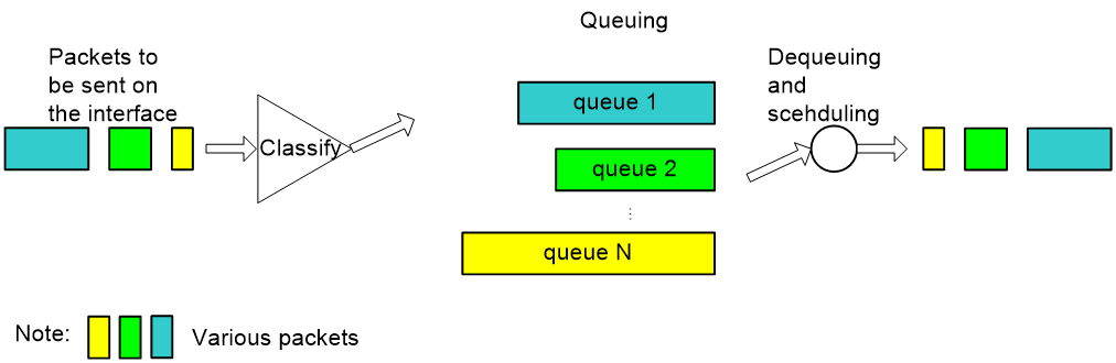
A device’s support for QoS is implemented by the combination of various QoS technologies. Figure 1 describes the processing sequence of QoS technologies.
Figure 1 Processing sequence of QoS technologies on a network device
Figure 1 briefly describes how the QoS module processes traffic.
1. Traffic classifier identifies and classifies traffic for subsequent QoS actions.
2. The QoS module takes various QoS actions on classified traffic as configured, depending on the traffic processing phase and network status. For example, you can configure the QoS module to perform the following operations:
¡ Traffic policing for incoming traffic.
¡ Traffic shaping for outgoing traffic.
¡ Congestion avoidance before congestion occurs.
¡ Congestion management when congestion occurs.
Traffic classification and marking
Traffic classification assigns data packets with different priorities or into different classes. You can configure match criteria based on not only IP precedence or DSCP value of IP packets, and CoS value of 802.1p packets, but also incoming interface, source IP address, destination address, MAC address, IP protocol, or application port number. You can define a class for packets with a common quintuple of source IP address, source port number, protocol number, destination IP address, and destination port number, or for all packets destined for a certain network segment.
The downstream network can either adopt the classification results of its upstream network or re-classify the packets according to its own match criteria.
The following sections describe how to classify and mark traffic in IPv4, IPv6, and Layer-2 Ethernet networks.
IPv4 QoS traffic classification
Figure 2 shows the position of IP precedence and DSCP in the IP header.
IP precedence-based traffic classification
The ToS field in the IP header defines eight IP service classes, as shown in Table 1.
Table 1 Description on the eight IP service classes
|
Service type |
IP precedence |
|
Network Control |
7 |
|
Internet work Control |
6 |
|
CRITIC/ECP |
5 |
|
Flash Override |
4 |
|
Flash |
3 |
|
Immediate |
2 |
|
Priority |
1 |
|
Routine |
0 |
DSCP-based traffic classification
The DiffServ model defines 64 service classes, and some typical ones are described in Table 2.
Table 2 Description on typical DSCP PHBs
|
Service type |
DSCP PHB |
DSCP value |
|
Network Control |
CS7 (111000) |
56 |
|
IP Routing |
CS6 (110000) |
48 |
|
Interactive Voice |
EF (101110) |
46 |
|
Interactive Video |
AF41 (100010) |
34 |
|
Video control |
AF31 (011010) |
26 |
|
Transactional/interactive (corresponding to high-priority applications) |
AF2x (010xx0) |
18, 20, 22 |
|
Bulk Data (corresponding to medium-priority applications) |
AF1x (001xx0) |
10, 12, 14 |
|
Streaming Video |
CS4 (000100) |
4 |
|
Telephony Signaling |
CS3 (000011) |
3 |
|
Network Management |
CS2 (000010) |
2 |
|
Scavenger |
CS1 (000001) |
1 |
|
Best Effort |
0 |
0 |
IPv6 QoS traffic classification
The IPv6 header has a TC field similar to the Type of Service (ToS) field in the IPv4 header. IPv6 can thus provide differentiated QoS services for IP networks as IPv4 does and allows traffic classification and marking based on the IPv6 ToS field. At the same time, a 20-byte flow label field is added to the IPv6 header for future extension.
Ethernet QoS traffic classification
As shown in Figure 3, the VLAN tag field in the Ethernet frame header defines eight CoS priorities.
To which queue a service is mapped affects the delay, jitter, and bandwidth of the service. Table 3 describes the eight service classes in Ethernet.
Table 3 Description on the eight Ethernet services classes
|
Service type |
Service features |
Ethernet CoS |
Example applications |
|
Network Control |
Applicable to reliable transmission of network maintenance and management packets requiring low packet loss rate |
7 |
BGP, PIM, SNMP |
|
Internet work Control |
Applicable to transmission of network protocol control packets requiring low packet loss rate and low delay in large-scale networks |
6 |
STP, OSPF, RIP |
|
Voice |
Applicable to voice traffic, which generally requires a delay less than 10 ms |
5 |
SIP, MGCP |
|
Video |
Applicable to video traffic, which generally requires a delay less than 100 ms |
4 |
Real-Time Transport Protocol (RTP) |
|
Critical Applications |
Applicable to services requiring assured minimum bandwidth |
3 |
NFS, SMB, RPC |
|
Excellent Effort |
Also referred to as CEO’s best effort, which has a slightly higher priority than the best effort service and is used by a common information organization to deliver information to the most important customers |
2 |
SQL |
|
Best Effort |
The default service class, applicable to traffic requiring best-effort rather than preferential transmission |
1 |
HTTP, IM, X11 |
|
Background |
Applicable to bulk transfers that are permitted on the network but should not impact the use of the network by other users and critical applications |
0 |
FTP, SMTP |
The queue to which a service is assigned determines the delay, jitter, and bandwidth that can be achieved for the service.
Table 4 presents the service-to-queue mappings recommended by IEEE 802.1Q.
Table 4 Service-to-queue mappings recommended by IEEE 802.1Q
|
Number of queues |
Queue ID |
Service type |
|
1 |
1 |
Best effort, background, excellent effort, critical applications, voice, video, internet work control, network control |
|
2 |
1 |
Best effort, background, excellent effort, critical applications |
|
2 |
Voice, video, internet work control, network control |
|
|
3 |
1 |
Best effort, background, excellent effort, critical applications |
|
2 |
Voice, video |
|
|
3 |
Network control, Internet work control |
|
|
4 |
1 |
Best effort, background |
|
2 |
Critical applications, excellent effort |
|
|
3 |
Voice, video |
|
|
4 |
Network control, Internet work control |
|
|
5 |
1 |
Best effort, background |
|
2 |
Critical applications, excellent effort |
|
|
3 |
Voice, video |
|
|
4 |
Internet work control |
|
|
5 |
Network control |
|
|
6 |
1 |
Background |
|
2 |
Best effort |
|
|
3 |
Critical applications, excellent effort |
|
|
4 |
Voice, video |
|
|
5 |
Internet work control |
|
|
6 |
Network control |
|
|
7 |
1 |
Background |
|
2 |
Best effort |
|
|
3 |
Excellent effort |
|
|
4 |
Critical applications |
|
|
5 |
Voice, video |
|
|
6 |
Internet work control |
|
|
7 |
Network control |
|
|
8 |
1 |
Background |
|
2 |
Best effort |
|
|
3 |
Excellent effort |
|
|
4 |
Critical applications |
|
|
5 |
Video |
|
|
6 |
Voice |
|
|
7 |
Internet work control |
|
|
8 |
Network control |
Congestion management
Figure 4 Example diagram for congestion in a network
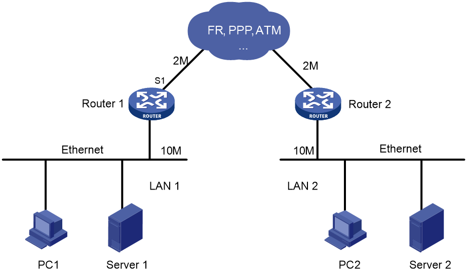
In computer data communications, communication channels are shared by computers. Additionally, the bandwidth of a WAN is usually smaller than that of a LAN. Because of this, the data sent from one LAN to another LAN cannot be transmitted in the WAN at the same rate as in the LANs. Bottlenecks prone to congestion are thus created at the forwarding devices between the LANs and the WAN. As shown in Figure 4, when LAN 1 sends data to LAN 2 at 10 Mbps, serial interface S1 of Router 1 will be congested.
Congestion management deals with traffic management and control during times of congestion. To this end, congestion management uses queuing technologies to create queues, classify packets, assign different classes of packets to different queues, and schedule queues. An uncongested interface sends out packets as soon as they are received. When the arriving rate is greater than the sending rate on the interface, congestion occurs. Then, congestion management classifies arriving packets and assigns them to different queues and queue scheduling processes these packets based on the priority and processes high-priority packets preferentially. Common queuing technologies include FIFO, PQ, CQ, WFQ, CBWFQ, and RTP priority queuing. The following section will describe these queuing mechanisms.
FIFO
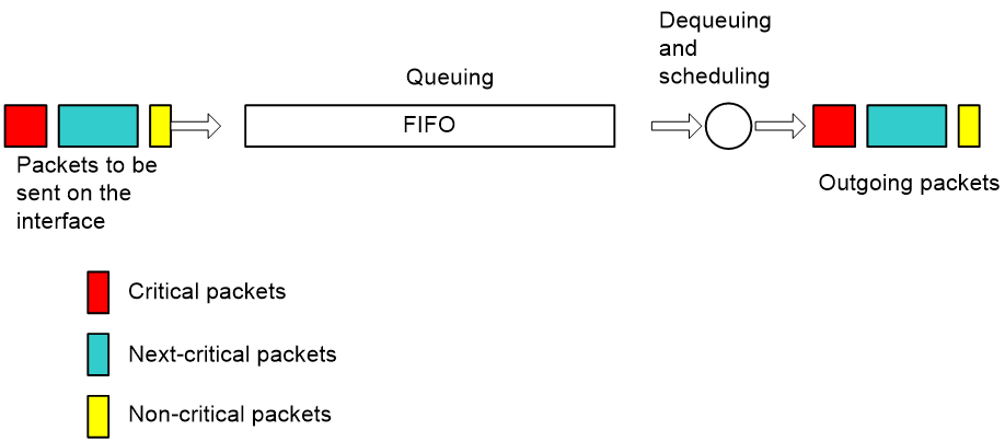
As shown in Figure 5, First in First Out (FIFO) does not classify packets. When the arriving rate is greater than the sending rate on the interface, FIFO enqueues and dequeues packets in the order the packets arrive.
As shown in Figure 4, suppose Server 1 in LAN 1 sends mission-critical data to Server 2 in LAN 2 and PC 1 in LAN 1 sends non-critical traffic to PC 2 in LAN 2. FIFO dequeues the packets of the two traffic flows in their arriving order without considering whether they are critical or not.
PQ
Figure 6 Schematic diagram for PQ
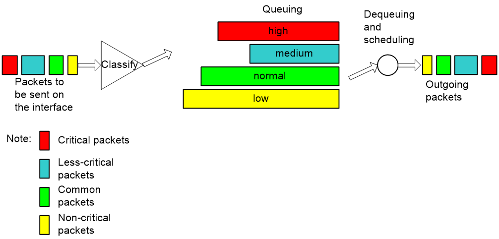
As shown in Figure 6, Priority Queuing (PQ) classifies packets. In an IP network, PQ classifies packets according to match criteria such as IP precedence, DSCP values, and IP quintuples; in a Multiprotocol Label Switching (MPLS) network, PQ classifies packets according to EXP values. PQ classifies packets into up to four classes, each corresponding to one of the four priority queues, and assigns each class of packets to the corresponding queue. The four priority queues are the top queue, middle queue, normal queue, and bottom queue in the descending order of priority. When dequeuing packets, PQ sends packets in the top queue first and dequeues a queue only when no packets are waiting for transmission in the higher priority queue. When congestion occurs, packets in higher-priority queues preempt packets in lower-priority queues to be transmitted. Thus, high-priority traffic, VoIP traffic, for example, is always processed preferentially while low-priority traffic, E-mail traffic, for example, is processed only when there is no mission-critical traffic in the network. PQ thus fully utilizes network resources while ensuring preferential transmission for high-priority services.
As shown in Figure 4, suppose traffic from Server 1 in LAN 1 to Server 2 in LAN 2 is mission critical, and traffic from PC 1 in LAN 1 to PC 2 in LAN 2 is not critical. Enable PQ on serial interface S1 of Router, and configure to assign traffic between servers to a high-priority queue and traffic between PCs to a low-priority queue. Then, PQ will provide differentiated services for the two traffic flows to transmit traffic between the servers preferentially, and transmit traffic between the PCs when there is no traffic between the servers in the network.
CQ
Figure 7 Schematic diagram for CQ
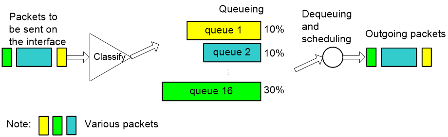
As shown in Figure 7, Custom Queuing (CQ) classifies packets. In an IP network, CQ classifies packets according to match criteria such as IP precedence, DSCP values, and IP quintuples; in an MPLS network, PQ classifies packets according to EXP values. CQ classifies packets into up to 16 classes, each corresponding to one of the 16 custom queues, and assigns each class of packets to the corresponding queue. You can assign a certain percentage of interface bandwidth to each custom queue. When dequeuing packets, CQ takes packets out of the custom queues by bandwidth percentage and then sends them out the interface.
Comparing CQ with PQ, you can see:
· PQ gives high-priority queues absolute preferential treatment over low-priority queues to ensure that mission-critical services are always processed preferentially. However, when the arriving rate of high-priority packets is always greater than the sending rate of the interface, low-priority packets can never be served. Using CQ, you can avoid this problem.
· CQ assigns a certain percentage of the interface bandwidth to each queue. In this way, CQ assigns bandwidth to traffic of different services proportionately to ensure that non-critical services can get served while mission-critical services enjoy more bandwidth. However, as CQ schedules queues cyclically, its delay guarantee for high-priority services, especially real-time services, is not as good as that of PQ.
As shown in Figure 4, suppose Server 1 in LAN 1 sends mission-critical data to Server 2 in LAN 2 and PC 1 in LAN 1 sends non-critical traffic to PC 2 in LAN 2. You can configure CQ on serial interface S1 of Router to perform congestion management as follows:
· Assign the traffic between the servers to queue 1, and allocate 60% of the interface bandwidth to queue 1, enabling the device to schedule 6000 bytes of packets from the queue in a cycle of scheduling for example.
· Assign the traffic between the PCs to queue 2, and allocate 20% of the interface bandwidth to queue 2, enabling the device to schedule 2000 bytes of packets from the queue in a cycle of scheduling for example.
· Allocate 20% of the interface bandwidth to packets in the other queues, enabling the device to schedule 2000 bytes of packets from the queue in a cycle of scheduling for example.
Thus, the traffic between the servers and the traffic between the PCs are treated differently. CQ schedules the queues cyclically. It first takes and sends out no less than 6000 bytes in queue 1, then no less than 2000 bytes in queue 2, and at last schedules the other queues. The bandwidth is assigned as follows:
· The physical bandwidth of serial interface S1 of Router 1 is 2 Mbps, of which the mission-critical data can occupy at least 2 × 0.6 = 1.2 Mbps of bandwidth, and the non-critical data can occupy at least 2 × 0.2 = 0.4 Mbps of bandwidth.
· When only the two data flows are sent out S1, the remaining free physical bandwidth of serial interface S1 is proportionally shared by the two data flows, that is, the mission-critical data can occupy at least 2 × 0.6/(0.2 + 0.6) = 1.5 Mbps of bandwidth, and the non-critical data can occupy at least 2 × 0.2/(0.2 + 0.6) = 0.5 Mbps of bandwidth.
· When only non-critical data is sent out S1, the non-critical data can occupy 2 Mbps of bandwidth.
WFQ
As shown in Figure 8, Weighted Fair Queuing (WFQ) classifies packets by flow. In an IP network, packets belong to the same flow if they have the same source IP address, destination IP address, source port, destination port, protocol number, and IP precedence (or DSCP value). In an MPLS network, packets with the same EXP value belong to the same flow. WFQ assigns each flow to a queue, and tries to assign different flows to different flows. The number of WFQ queues (represented by N) is configurable. When dequeuing packets, WFQ assigns the outgoing interface bandwidth to each flow by IP precedence, DSCP value, or EXP value. The higher the precedence of a flow is, the higher bandwidth the flow gets. Based on fair queuing, WFQ assigns weights to services of different priorities.
For example, assume that there are eight flows on the current interface, with the precedence being 0, 1, 2, 3, 4, 5, 6, and 7 respectively. The total bandwidth quota is the sum of all the (precedence value + 1)s, that is, 1 + 2 + 3 + 4 + 5 + 6 + 7 = 36. The bandwidth percentage assigned to each flow is (precedence value of the flow + 1)/total bandwidth quota. That is, the bandwidth percentage for each flow is 1/36, 2/36, 3/36, 4/36, 5/36, 6/36, 7/36, and 8/36.
Look at another example. Assume there are four flows in total, and priority value 4 is assigned to three flows and 5 to one flow. Then the total bandwidth quota is (4 + 1) × 3 + (5 + 1) = 21. Thus, each flow with priority 4 will occupy 5/21 of the total bandwidth and the one with priority 5 will occupy 6/21 of the total bandwidth.
Thus, WFQ assigns different scheduling weights to services of different priorities while ensuring fairness between services of the same priority
CBWFQ
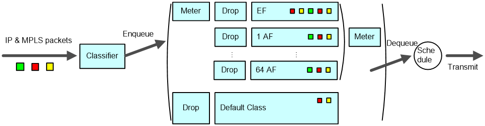
As shown in Figure 9, class-based WFQ (CBWFQ) classifies packets according to match criteria such as IP precedence, DSCP values, and IP quintuples in an IP network or according to EXP values in an MPLS network, and then assigns different classes of packets to different queues. Packets that do not match any class are assigned to the system-defined default class.
CBWFQ defines three types of queues: EF, AF, and BE. This section introduces the three queue types.
EF queue
As shown in Figure 9, the EF queue (or low latency queue, (LLQ)) is a high-priority queue. One or multiple classes of packets can be assigned to the EF queue and each assigned a certain amount of bandwidth to create an EF queue instance. When dequeuing packets, CBWFQ sends packets (if any) in the EF queue preferentially, and then packets in the other queues when the EF queue is empty or when the bandwidth assigned to the EF queue exceeds the configured maximum reserved bandwidth.
When the interface is not congested (that is, all queues are empty), all packets arriving at the EF queue will be sent. When the interface is congested, that is, when there are packets waiting for transmission in queues, the EF queue will be rate-limited and the packets in the EF queue exceeding the defined specifications will be dropped. Thus, packets in the EF queue can use free bandwidth, but will not occupy the bandwidth exceeding the specifications. In this way, due bandwidth of other packets is protected. Additionally, once a packet arrives at the EF queue, it will be dequeued. Therefore, the maximum delay for packets in the EF queue is the time used for sending a packet of the maximum length. The packets in the EF queue thus enjoy the minimum delay and jitter. This guarantees QoS for delay-sensitive applications such as VoIP.
As rate limiting takes effect on the EF queue when the interface is congested, you do not need to set the EF queue length. Because packets in the EF queue are generally VoIP packets encapsulated in UDP, you may use the tail drop policy instead of the weighted random early detection (WRED) drop policy.
AF queue
As shown in Figure 9, AF queues 1 through 64 each accommodate a class of packets and represent a certain amount of bandwidth that is user assigned. The AF queues are scheduled by assigned bandwidth. CBWFQ ensures fairness between different classes of packets. When a certain class does not have packets waiting for transmission, the AF queues can fairly share the free bandwidth. Compared with the time division multiplexing (TDM) system, this mechanism improves link efficiency. When the interface is congested, each class of packets is guaranteed of minimum bandwidth administratively assigned.
For an AF queue, when the queue length reaches the maximum length, tail drop is used by default, but you can configure to use WRED drop instead. For detailed information about WRED drop, refer to the section describing WRED.
BE queue
Packets that do not match any user-defined class are assigned to the system-defined default class. Even though you can assign the default class to an AF queue to assign bandwidth for the class, the default class is assigned to the BE queue in most cases. WFQ is used to schedule the BE queue; thus, all packets of the default class are scheduled based on flows.
For the BE queue, when the queue length reaches the maximum length, tail drop is used by default, but you can configure WRED drop instead. For detailed information about WRED drop, refer to the section describing WRED.
Use of the three queues
To sum up,
· The low-delay EF queue is used to guarantee EF class services of absolute preferential transmission and low delay.
· The bandwidth guaranteed AF queues are used to guarantee AF class services of assured bandwidth and controlled delay.
· The default BE queue is used for BE class services and uses the remaining interface bandwidth for sending packets.
The packets entering the EF queue and AF queues must be metered. Considering the overheads of the Layer-2 headers and physical layer overheads (such as the ATM cell header), you are recommended to assign no more than 80% of the interface bandwidth to the EF queue and AF queues.
RTP priority
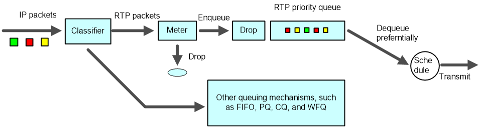
RTP priority queuing is a simple queuing technology designed to guarantee QoS for delay-sensitive real-time services (including voice and video services). It assigns RTP packets carrying voice or video to a high-priority queue for preferential treatment, thus minimizing the delay and jitter and ensuring QoS for voice or video services.
As shown in Figure 10, RTP priority queuing assigns RTP packets to a high-priority queue. An RTP packet is a UDP packet with an even destination port number in the valid range, usually 16384 to 32767. RTP priority queuing can be used in conjunction with any queuing method from FIFO, PQ, CQ, WFQ, to CBQ, while it always has the highest priority. You are not recommended to use RTP priority queuing in conjunction with CBWFQ however, because low latency queuing (LLQ) of CBWFQ can provide sufficient QoS guarantee for real-time services.
The rate of packets entering the RTP priority queue is limited, and the packets exceeding the specifications are dropped. In this way, when the interface is congested, the RTP priority queue will not occupy more bandwidth than defined. Ensuring the due bandwidth of other packets, RTP priority queuing addresses the problem that queues other than the RTP priority queue may be starved.
Congestion management technology comparison
Table 5 Congestion management technology comparison
|
Queue name |
Number of queues |
Advantages |
Disadvantages |
|
FIFO |
1 |
· No need to configure, easy to use · Simple processing procedure, low delay |
· All packets are treated equally. The available bandwidth, delay, and drop probability are determined by the arrival order of the packets. · No restriction on incooperative data sources (that is, flows without the flow control mechanism, UDP for example), resulting in bandwidth loss of cooperative data sources such as TCP. · No delay guarantee for delay-sensitive real-time applications, such as VoIP. |
|
PQ |
4 |
Provide absolute priority and delay guarantees for real-time and mission-critical applications such as VoIP |
· Need to be configured; low processing speed. · No restriction is imposed on the bandwidth assigned to the high-priority queues, low-priority packets may fail to get bandwidth. |
|
CQ |
16 |
· Assign different bandwidth percentages to different services · When packets of certain classes are not present, their bandwidth can be shared by packets of other classes |
· Need to be configured; low processing speed · Not applicable to delay-sensitive real-time services |
|
WFQ |
Configurable |
· Easy to configure, automatic traffic classification · Bandwidth guarantee for packets from cooperative (interactive) sources such as TCP · Reduced jitter · Reduced delay for interactive applications that feature small traffic size · Proportional bandwidth assignment for traffic flows of different priorities · As the number of traffic flows decreases, bandwidth for the existing flows increases automatically. |
· The processing speed is faster than that of PQ and CQ but slower than that of FIFO · Not applicable to delay-sensitive real-time services |
|
RTPQ |
1 |
Cooperate with other queuing mechanisms to provide absolutely preferential scheduling for low-delay traffic such as VoIP traffic |
Less classification options than CBWFQ |
|
CBWFQ |
Configurable |
· Flexibly classify traffic based on various criteria and provide different queue scheduling mechanisms for EF, AF and BE services. · Provide a highly precise bandwidth guarantee and queue scheduling on the basis of AF service weights for various AF services. · Provide absolutely preferential queue scheduling for the EF service to meet the delay requirement of real-time data; overcome the disadvantage of PQ that some low-priority queues are not serviced by restricting high-priority traffic. · Provide flow-based WFQ scheduling for best-effort default-class traffic. |
The system overhead grows as the number of classes increases. |
Congestion avoidance
Serious congestion causes great damages to network resources. Measures must be taken to avoid congestion. Congestion avoidance is a flow control mechanism. It monitors utilization of network resources (such as queues or memory buffers) and actively drops packets when congestion deteriorates to prevent network overload.
Compared to point-to-point flow control, this flow control mechanism is of broader sense because it controls the load of more flows on a device. When dropping packets, the device can still cooperate well with the flow control mechanism (such as TCP flow control) performed at the source station to better adjust network traffic to a reasonable size. The cooperation of the packet drop policy at the device and the flow control mechanism at the source station can maximize the throughput and utilization rate of the network and minimize packet loss and delay.
Traditional packet drop policy
The traditional packet drop policy is tail drop. When the queue length reaches the maximum threshold, all the subsequent packets are dropped.
Tail drop can result in global TCP synchronization. That is, if packets of multiple TCP connections are dropped at the same time, these TCP connections go into the state of congestion avoidance and slow start to reduce traffic and then come back at the same time to cause another traffic peak. This causes oscillation between peaked congestion and off congestion on the network.
RED and WRED
You can use random early detection (RED) or weighted random early detection (WRED) to avoid global TCP synchronization.
The RED or WRED algorithm sets an upper threshold and lower threshold for each queue, and processes the packets in a queue as follows:
· When the queue size is shorter than the lower threshold, drop no packets;
· When the queue size reaches the upper threshold, drop all subsequent packets;
· When the queue size is between the lower threshold and the upper threshold, drop received packets at random. The longer a queue is, the higher the drop probability is. However, a maximum drop probability exists.
If the current queue size is compared with the upper threshold and lower threshold to determine the drop policy, bursty traffic is not fairly treated. To solve this problem, WRED compares the average queue size with the upper threshold and lower threshold to determine the drop probability. The average queue size is calculated using the formula: average queue size = previous average queue size × (1 – 2-n) + current queue size × 2-n, where n is configurable. The average queue size reflects the queue size change trend but is not sensitive to bursty queue size changes, and thus bursty traffic can be fairly treated.
Different from RED, WRED determines differentiated drop policies for packets with different IP precedence values, DSCP values, or EXP values. With WRED, packets with a lower IP precedence are more likely to be dropped. If you configure the same drop policy for all priorities, WRED functions as RED.
Both RED and WRED avoid global TCP synchronization by randomly dropping packets. When the sending rate of a TCP session slows down after its packets are dropped, the other TCP sessions remain in high sending rates. Because there are always TCP sessions in high sending rates, link bandwidth use efficiency is improved.
Relationship between WRED and queuing mechanism
The relationship between WRED and queuing mechanism is shown in Figure 11:
Figure 11 Relationship between WRED and queuing mechanism
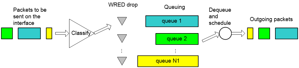
When the queuing mechanism is WFQ,
· you can set the exponent for average queue size calculation, upper threshold, lower threshold, and drop probability for packets of different priorities respectively to provide different drop policies.
· you can realize flow-based WRED. Each flow has its own queue after classification. Because the queue length of a small-sized flow is shorter than a large-sized flow, the small-sized flow will have lower packet drop probability. In this way, the interests of small-sized flows are protected.
By using WRED in conjunction with FIFO, PQ, or CQ:
· you can set the exponent for average queue length calculation, upper threshold, lower threshold, and drop probability for each queue to provide differentiated drop policies for packets in different queues.
· you ensure that the smaller a flow is, the lower its drop probability is statistically, thus protecting the interests of small-sized flows.
Traffic shaping and traffic policing
Traffic policing typically limits a connection's traffic and busty traffic entering the network. If the packets of a certain connection exceed the specifications, traffic policing drops the exceeding packets or re-marks precedence for the exceeding packets depending on your configuration. Typically, committed access rate (CAR) is used for limiting a certain type of traffic. For example, you can set the maximum bandwidth allocated to HTTP packets to 50% of the total bandwidth.
Traffic shaping typically limits a connection's traffic and busty traffic leaving the network to smooth the traffic sending rate. Generally, traffic shaping is implemented by buffers and token buckets. When the sending rate of packets is too high, packets are buffered, and then sent out at an even rate under the control of token buckets.
CAR
For an ISP, it is necessary to limit the rate of upstream traffic from customers. For an enterprise network administrator, limiting the traffic rates of certain applications is an effective way of controlling network performance. CAR can help them control traffic effectively.
CAR uses token buckets for traffic control.
Figure 12 Flow chart of CAR performing traffic control
Figure 12 shows how CAR controls traffic. At first, CAR classifies packets based on pre-define match criteria, delivers the unmatched packets directly without regulating them with the token bucket, and sends the matched packets to the token bucket for processing. The token bucket is a tool for traffic control. The system puts tokens into the bucket at the set rate. You can set the capacity of the token bucket. When the token bucket is full, extra tokens overflow and the number of tokens in the bucket stops increasing. The number of tokens in the bucket indicates the traffic size that can be lent to bursty traffic. If the token bucket has enough tokens for sending packets, then the packets are forwarded, and accordingly, the tokens used for forwarding are removed from the token bucket. If the token bucket does not have enough tokens, the packets are dropped. Packets can be sent after new tokens are generated in the token bucket. Thus, by restricting traffic rate to the rate of generating tokens, traffic control is implemented.
In actual applications, CAR can be used not only for traffic control, but also for marking or re-marking packets. That is, CAR can be used to set IP precedence or modify IP precedence for IP packets. For example, you can use CAR to set the precedence of packets meeting the match criteria to 5, and drop the packets not meeting the match criteria or set the precedence of the packets to 1 and continue to send them. Thus, the subsequent processing module will try to guarantee transmission of packets with precedence 5, and send packets with precedence 1 when the network is not congested; when the network is congested, it will drop packets with precedence 1 prior to packets with precedence 5.
Additionally, CAR allows you to classify traffic multiple times. For example, you can limit part of the traffic to certain specifications, and then limit all traffic.
GTS
Generic traffic shaping (GTS) provides measures to adjust the rate of outbound traffic actively. A typical traffic shaping application is to adapt the local traffic output rate to the downstream traffic policing parameters.
Like CAR, GTS uses token buckets for traffic control. The difference between GTS and CAR is that packets to be dropped by CAR are buffered in GTS. Therefore, GTS decreases the number of packets dropped caused by bursty traffic.
Figure 13 is the processing flow of GTS. The queue used for buffering packets is called the GTS queue.
GTS can shape traffic as a whole or on a per-flow basis on an interface. When packets arrive, GTS classifies the packets based on the pre-define match criteria, forwards the unmatched packets directly without processing them with the token bucket, and sends the matched packets to the token bucket for processing. The token bucket generates tokens at the pre-defined rate. If the token bucket has enough tokens, the packets are forwarded, and at the same time, the tokens used for transmission are removed from the token bucket. If the token bucket does not have enough tokens, GTS buffers the packets in the GTS queue, and enqueues the packets subsequently received after detecting packets in the GTS queue. If the GTS queue length reaches the upper limit, newly arriving packets are dropped directly. GTS dequeues packets in the GTS queue regularly. For each packet transmission, GTS checks the number of tokens in the token bucket to make sure that enough tokens are available. GTS stops transmitting packets when tokens in the token bucket are not enough for sending packets or no packet is buffered in the GTS queue.
As shown in Figure 4, to reduce the number of packets dropped because of bursty traffic, you can enable GTS on the egress interface of Router 1. The packets exceeding the GTS specifications are buffered on Router A. When the next transmission is allowed, GTS takes out the buffered packets and sends them. In this way, all the traffic sent to Router 2 conforms to the traffic specifications defined by Router 2, and the number of packets dropped on Router 2 is reduced. Comparatively, if you do not enable GTS on the egress interface of Router 1, all packets exceeding the CAR specifications configured on Router 2 will be dropped by Router 2.
Line rate
The line rate (LR) of a physical interface specifies the maximum forwarding rate of the interface. The limit does not apply to critical packets.
Line rate also uses token buckets for traffic control. With line rate configured on an interface, all packets to be sent through the interface are first handled by the token bucket at line rate. When enough tokens are available, packets are forwarded; otherwise, packets are put into QoS queues for congestion management. In this way, line rate controls the traffic passing through a physical interface.
Figure 14 Line rate implementation
Figure 14 shows the processing flow of line rate. As line rate uses a token bucket for traffic control, bursty traffic can be transmitted so long as enough tokens are available in the token bucket. If tokens are inadequate, packets cannot be transmitted until the required tokens are generated in the token bucket. Line rate thus limits traffic rate to the rate of generating tokens while allowing bursty traffic. Because line rate does not classify packets, it is a good approach when you only want to limit the rate of all packets.
Line rate can use rich QoS queues to buffer exceeding packets, while GTS can buffer them only in the GTS queue.
Link efficiency mechanisms
Link efficiency mechanisms can improve the QoS level of a network by improving link performance. For example, they can help reduce the packet transmission delay of a link for a specific service and adjust available bandwidth.
Link fragmentation & interleaving (LFI) and IP header compression (IPHC) are two link efficiency mechanisms in common use.
LFI
On a slow link, even if you assign real-time traffic (VoIP traffic) to a high priority queue (RTP priority queue or LLQ queue for example), you cannot guarantee the traffic of low delay or jitter because voice packets must wait for transmission when the interface is sending other data packets, which tends to take a long time on the slow link. With LFI, data packets (packets which are not in the RTP priority queue or LLQ) are fragmented before transmission and transmitted one by one. When voice packets arrive, they are transmitted preferentially. In this way, the delay and jitter are decreased for real-time applications. LFI is applicable to slow links.
As shown in Figure 15, with LFI, when large packets are dequeued, they are fragmented into small fragments of the customized length. When a packet is put into the RTP priority queue or LLQ queue while a fragment is being sent, it does not have to wait a long time for its turn as it would without LFI. In this way, the delay caused by transmitting large packets over a slow link is greatly reduced.
IPHC
The Real Time Protocol (RTP) can carry real-time multimedia services, such as voice and video, over IP networks. An RTP packet comprises a large header portion and relatively small payload. The header of an RTP packet includes a 12-byte RTP header, 20-byte IP header, and 8-byte UDP header. The IP/UDP/RTP header is thus of 40 bytes in total, while a typical RTP payload is only of 20 bytes to 160 bytes. To avoid unnecessary bandwidth consumption, you can use the IP header compression (IPHC) feature to compress the headers. After compression, the 40-byte header can be squeezed into 2 to 5 bytes. Without the checksum, the header can be squeezed into 2 bytes. If the payload is of 40 bytes and the header is squeezed into 5 bytes, the compression ratio is (40+40) / (40+5), about 1.78, which is very efficient. IPHC can effectively reduce bandwidth consumption on links, especially on slow links, to improve link efficiency.
Implementation of MPLS QoS
Currently, IP networks support only the DiffServ model, while MPLS networks support both the DiffServ model and the IntServ model.
· The principle of DiffServ is the same in both MPLS networks and IP networks except that in MPLS networks, the DiffServ PHBs are implemented through the EXP field in the MPLS header.
· IntServ in an MPLS network is implemented by MPLS TE.
This section briefly introduces the two MPLS QoS technologies.
MPLS DiffServ
With DiffServ in an IP network, traffic is classified into service classes according to QoS requirements at the edge of the network, and the service class of a packet is uniquely identified by the DS field in the ToS field of its IP header; then, the nodes that the packet traverses in the backbone network look at the DS field to apply the QoS policy predefined for the service class. Traffic classification and marking in DiffServ is similar to MPLS label distribution. In fact, MPLS-based DiffServ is implemented by combining DS marking with MPLS label distribution.
MPLS DiffServ is implemented by using the EXP field in the MPLS header to carry DiffServ PHBs. A label switching router (LSR) makes forwarding decisions based on the MPLS EXP. The problem is how to map 64 DiffServ PHBs to the 3-bit EXP field. MPLS DiffServ provides two solutions to address the problem. You can choose either solution depending on your network environments.
· One is the EXP-inferred-Label Switched Paths (E-LSP) solution, which uses EXP bits to signal the PHB treatment for individual packets on an LSP. This solution is applicable to networks supporting no more than eight PHBs. This solution directly maps DSCP values to EXP values for identifying the specific PHBs. For an MPLS packet, its label decides the LSP that it travels and its EXP value decides its scheduling priority and drop precedence at every LSR hop. An LSP can thus carry up to eight classes of traffic with different PHBs. The operator can configure the EXP values directly or map DSCP values to EXP values. This solution does not require the signaling protocol to signal PHB information, and allows efficient use and status maintenance of labels.
· The other is the label-inferred LSPs (L-LSP) solution, which uses both labels and EXP bits to decide PHB treatment of packets on an LSP. This solution is applicable to networks supporting more than eight PHBs. For an MPLS packet, its label decides not only the LSP that it travels but also the scheduling behavior on the LSP, while the EXP bits decide only its drop precedence. Because labels are used for classifying traffic, you need to establish different LSPs for different flows. This solution uses more labels and maintains more state information than the E-LSP solution.
The H3C MPLS DiffServ implementation uses the E-LSP solution, where
· The EXP field is used to signal the PHB treatment of packets in an MPLS network, including the queue ID and drop precedence. You are recommended to configure the DiffServ PHB-to-EXP mappings as shown in Table 6.
· All DiffServ components (the traffic conditioner and various PHBs) are extended for EXP.
Table 6 Recommended DiffServ PHB-to-EXP mapping table
|
DSCP PHB |
EXP value |
|
CS7 (111000) |
111 |
|
CS6 (110000) |
110 |
|
EF (101110) |
101 |
|
AF4X (100xx0) |
100 |
|
AF3X (011xx0) |
011 |
|
AF2X (010xx0) |
010 |
|
AF1X (001xx0) |
001 |
|
Best Effort |
000 |
Figure 16 Mappings between DiffServ PHBs and EXP values
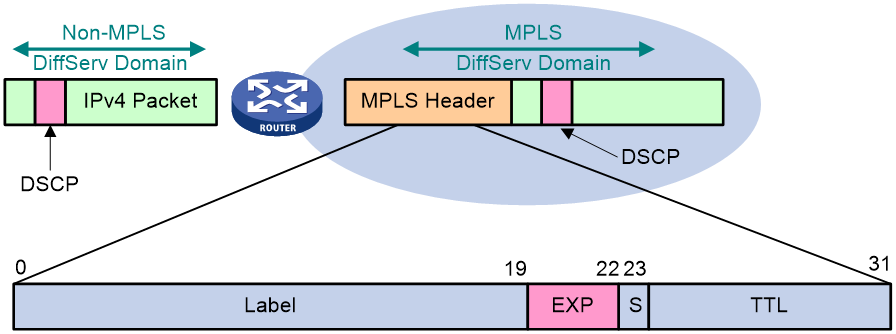
As shown in Figure 16, at the edge of the MPLS network, the IP precedence of IP packets are copied to the EXP field of MPLS packets directly by default. However, if the ISP does not trust the customer network or the DiffServ classes defined by the ISP are different from those of the customer network, you can classify packets based on such criteria as IP precedence, DSCP values, IP quintuple, and incoming interfaces, and then set new EXP values for MPLS packets at the edge of the MPLS network. In the MPLS network, the ToS field of IP packets remains unchanged.
The intermediate nodes in the MPLS network classify packets into different PHBs according to their EXP values to implement congestion management, traffic policing, or traffic shaping for them.
MPLS-TE
MPLS-TE is a technology that indirectly improves QoS for MPLS networks. Traditional routing protocols such as OSPF and IS-IS mainly aim to guarantee connectivity and reachability of networks, and thus generally select insensitive parameters to calculate SPF. This is prone to cause unbalanced traffic distribution and route flapping. MPLS-TE is intended to address partial network congestion caused by unbalanced load distribution. It achieves this by manipulating traffic dynamically to adapt to performance of limited physical network resources.
The performance objectives associated with traffic engineering can be either of the following:
· Traffic oriented. These are performance objectives that enhance QoS of traffic streams, such as minimization of packet loss, minimization of delay, maximization of throughput and enforcement of service level agreement (SLA).
· Resource oriented. These are performance objectives that optimize resources utilization. Bandwidth is a crucial resource on networks. Efficiently managing it is a major task of traffic engineering. MPLS TE combines MPLS with traffic engineering. It reserves resources by establishing LSP tunnels to specific destinations. This allows traffic to bypass congested nodes to achieve appropriate load distribution.
MPLS-TE can establish bandwidth-guaranteed paths for traffic flows. With MPLS-TE, you can configure bandwidth settings (maximum physical bandwidth and maximum reserved bandwidth) for each link. The bandwidth information will flood through an IGP to generate a TE database (TEDB). At the ingress of an LSP, you can assign bandwidth to it. Based on the constraints, CSPF calculates a path that meet the bandwidth, delay and other constraints for the LSP and RSVP-TE establishes the LSP according to the calculation results. For delay sensitive services like VoIP, you use link delay as a TE metric for path calculation.
In addition, MPLS-TE provides a mechanism to mark LSPs with priorities to allow a more-important LSP to preempt less-important LSPs. The mechanism allows you to use low-priority LSPs to reserve resources when no high priority LSPs are required but still ensures that high-priority LSPs are always established along the optimal path and not affected by resource reservation. MPLS-TE uses two priority attributes to make preemption decisions: setup priority and holding priority. Both setup and holding priorities range from 0 to 7, with a lower numerical number indicating a higher priority. The setup priority of an LSP decides whether the LSP can get required resources when it is first set up and the hold priority decides whether the LSP can hold when a new LSP comes up to competes with it. For the new LSP to preempt the existing LSP, the setup priority of the new LSP must be greater than the holding priority of the existing one.
MPLS-TE also provides the automatic bandwidth adjustment function to dynamically tune bandwidth assigned to an LSP to accommodate increased service traffic for example. The idea is to measure traffic size on a per-LSP basis, periodically check the actual bandwidth used by the LSPs, and tune bandwidth assignment automatically in a certain range.
Application scenarios
QoS implementation in an enterprise VPN
An ISP can provide virtual private network (VPN) services for enterprises over its IP network to reduce their costs in networking and leasing lines. For enterprises, this is very attractive. An enterprise can use VPNs to connect its traveling personnel, geographically distributed branches, business partners to the headquarters for communication. However, the benefits of VPNs will be offset if they fail to transmit data timely and effectively because of ineffective QoS assurance. Suppose an enterprise requires that the business contact letters and database access be prioritized and guaranteed of bandwidth, and business-irrelevant E-mails and WWW accesses treated as best-effort traffic.
You can use the rich set of QoS mechanisms provided by H3C to meet the requirements for enterprise VPNs:
· Mark IP precedence/DSCP values for different types of traffic, and classify traffic based on IP precedence/DSCP values.
· Use CBWFQ to guarantee QoS performance such as bandwidth, delay, and jitter for business data.
· Use the WRED/tail drop mechanism to treat VPN information differentially, avoiding traffic oscillation in the network;
· Use traffic policing to limit the traffic of each flow in the VPN.
On the CE router of each VPN site, classify and color traffic. For example, classify traffic into database access, critical business mails, and WWW access, and use CAR to mark the three classes with high priority, medium priority, and low priority respectively. At the same time, the VPN service provider can configure CAR and GTS on the access ports of each CE router to restrict the traffic entering the ISP network from each VPN site within the committed traffic specifications. In addition, you can configure line rate on CE routers to limit the total traffic rate of an interface. By controlling the bandwidth available on each access port, you can protect the interests of the VPN service provider.
On each PE router in the network of the VPN service provider, the IP precedence of IP packets is copied to the MPLS EXP field by default. Thus, you can configure WFQ and CBWFQ on PE and P routers in the VPN service provider network to control the scheduling mode of packets, and guarantee that high-priority packets are served preferentially with low delay and low jitter when congestion occurs. At the same time, you can configure WRED to avoid TCP global synchronization.
Additionally, if the ISP expects to define service levels different from those of the customer network, or the ISP does not trust the IP precedence of the customer network, the ISP can re-mark MLS EXP values at the ingress of PE routers as needed.
VoIP QoS network design
The basic VoIP QoS requirements are: packet loss ratio < 1%, end-to-end single-trip time < 150 ms (depending on coding technologies), and jitter < 30 ms. The bandwidth that a session requires varies from 21 kbps to 106 kbps depending on the sampling rate, compression algorithm, and Layer-2 encapsulation.
Consider the following points in your VoIP QoS network design:
1. Assign network bandwidth appropriately to guarantee service transmission.
Appropriate bandwidth assignment is key to QoS assurance. For example, to deliver good voice quality on an IP phone voice connection, you need to assign the connection bandwidth of 21 kbps to 106 kbps, depending on the codec algorithm. If a voice connection requires 21 kbps, then you should avoid using a 64 kbps link to carry four 21-kbps voice connections at the same time. When constructing a network, plan the network and assign bandwidth resources appropriately according to the service model, and consider bandwidth multiplexing depending on how often a service is used. If all network services are frequently used, consider stacking bandwidth. When making voice channel assignment for an ISP network, take into full consideration the amount of available bandwidth of the ISP.
2. Select an appropriate voice codec technology
There are multiple voice compression algorithms, which require different transmission bandwidth. When abundant bandwidth is available, you can use the G.711 compression algorithm, which delivers low compression ratio with little impact on voice quality but is transmission bandwidth demanding. When bandwidth is insufficient, you can use the G.729 compression algorithm, which requires less bandwidth at the cost of voice distortion.
3. Select appropriate QoS management technologies
To reduce the delay of voice packets, you can combine the following technologies:
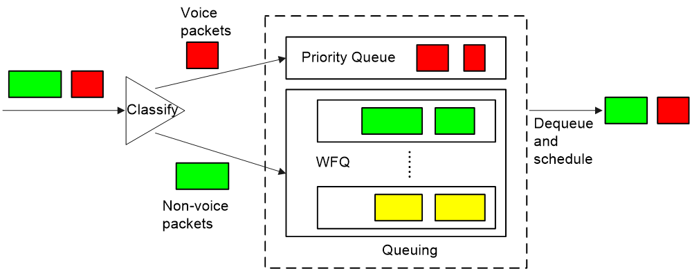
¡ Use the LLQ queue scheduling algorithm to assign voice packets to the LLQ queue to guarantee that voice packets are scheduled preferentially when congestion occurs. You can also combine RTP priority queuing with WFQ, as shown in Figure 17.
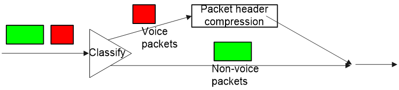
¡ Use the IPHC technology to improve link efficiency and reduce transmission delay, as shown in Figure 18.
¡ Use the LFI technology to reduce the delay of voice packets on slow links.
4. Deploy QoS at the access layer, distribution layer, and backbone layer.
¡ When planning services at the access layer, you can assign different services to different VLANs, for example, assign voice service traffic to VLAN 10, video service traffic to VLAN 20, and high-speed Internet access service traffic to VLAN 30. Thus, the devices at the access layer can apply its service transmission prioritization scheme based on VLANs to preferentially forward real-time services. If devices at the access layer do not support VLAN segmentation, you can assign voice traffic, video traffic, and high-speed Internet access traffic to different networks and isolate them at the physical layer. For example, you can assign IP addresses at different network segments to different kinds of service terminals.
¡ At the distribution layer, you can use different VPNs to guarantee bandwidth for voice services and video services. On a network not supporting VPN technology, you can classify traffic between the access layer and the distribution layer, assign higher priorities to voice traffic and video traffic than to data traffic, and then forward packets according to the priorities at the distribution layer, thus preventing bursty data traffic from affecting voice and video traffic.
¡ At the backbone layer, assign voice and video traffic to the same VPN to isolate it from the data traffic, thus guaranteeing QoS and security for voice and video services in the network. In the same VPN, you can further classify traffic and forward data packets according to their priorities. You can also combine VPN technology with MPLS technology to provide low-delay and bandwidth-guaranteed forwarding paths for voice services after assessing the overall resource conditions in the network.
References
· RFC 1349, Type of Service in the Internet Protocol Suite
· RFC 1633, Integrated Services in the Internet Architecture: an Overview
· RFC 2205, Resource Reservation Protocol (RSVP)-Version1 Functional Specification
· RFC 2210, The use of RSVP with IETF Integrated Services
· RFC 2211, Specification of the Controlled-Load Network Element Service
· RFC 2212, Specification of Guaranteed Quality of Service
· RFC 2215, General Characterization Parameters for Integrated Service Network Elements
· RFC 2474, Definition of the Differentiated Services Field (DS Field) in the IPv4 and IPv6 Headers
· RFC 2475, An Architecture for Differentiated Services
· RFC 2597, Assured Forwarding PHB Group
· RFC 2598, An Expedited Forwarding PHB (Per-Hop Behavior)
· RFC 2697, A single rate three color marker
· RFC 2698, A two rate three color marker
· RFC 3270, Multi-Protocol Label Switching (MPLS) Support of Differentiated Services
· IEEE 802.1Q-REV/D5.0 Annex G
